Causal Inference for Engineering Interventions
Workshop — 90 minutes
Causal Inference for Engineering Interventions
A hands-on workshop derived from Chapter 6 of Engineering Intelligence.
90 minutes · 4 hands-on segments
Learning outcomes
After this workshop you can:
Explain why before-after averages mislead
Draw a DAG for a proposed engineering intervention
Estimate an ATE and a CACE from cluster-randomised data
Compute a required sample size and a minimum detectable effect
Apply an O’Brien-Fleming boundary when you inspect an experiment repeatedly
The problem
Your organisation rolled out an AI reviewer. Review latency dropped from 8.4 hours to 5.9 hours. The vendor renewal is next week.
Did the tool cause the improvement?
Try to answer with what you already have. Notice how easy it is to fall for the naive answer.
The five alternative explanations
Quieter release period during the pilot
Repositories with simpler work adopted first
Reviewer staffing changed
CI became faster at the same time
Novelty effect from a shiny new tool
Naive comparison can’t rule any of them out.
Potential outcomes
For unit \(i\):
\(Y_i(1)\) = outcome with treatment
\(Y_i(0)\) = outcome without treatment
Individual effect \(\tau_i = Y_i(1) - Y_i(0)\)
The fundamental problem: you only observe one.
Every causal method is a strategy for estimating the missing counterfactual.
The DAG makes assumptions visible
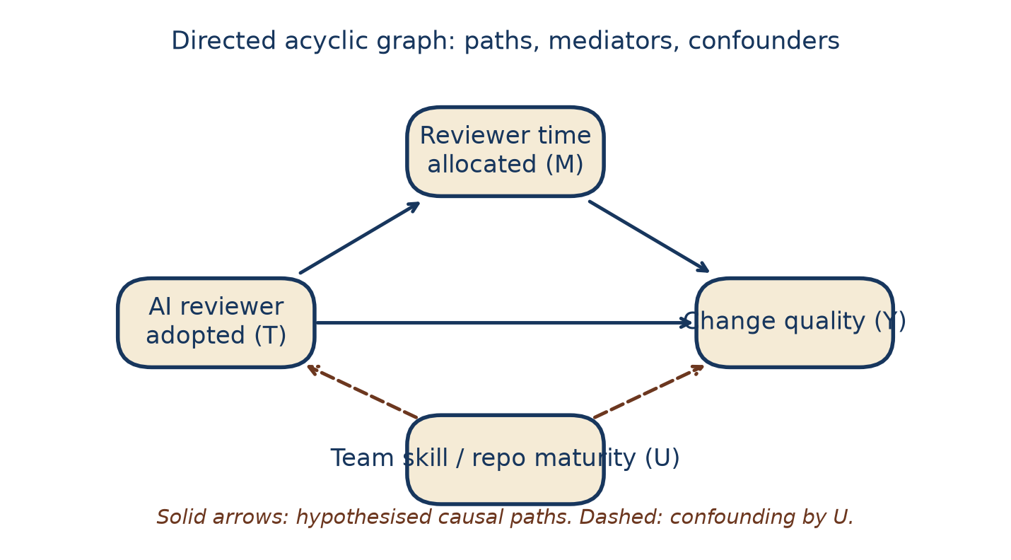
Where does randomising T help? Where must you adjust for U instead?
Segment 1 (15 min)
Draw the DAG for an intervention you’re actually considering.
Pair up. One partner draws. Other partner names the confounder they’d fear most. Swap.
Report back: share the confounder that would be hardest to adjust for.
Assignment vs analysis unit
Assignment unit — receives the treatment (team, repository, engineer)
Analysis unit — contributes an outcome (pull request, Engineering Change, service)
They can differ. Interference must be considered.
Pull-request assignment breaks down when reviewers are shared. Team-level assignment costs statistical power. Engineering-Change assignment is often the best match to the mechanism.
Difference-in-differences
For treated (T) and control © groups before/after:
Key assumption: parallel trends. Absent treatment, the two groups would have moved similarly.
Inspect pre-treatment trends. Report sensitivity.
The AI reviewer worked example
\(\bar{Y}_{T,\text{before}} = 5.6h\), \(\bar{Y}_{T,\text{after}} = 4.9h\)
\(\bar{Y}_{C,\text{before}} = 6.4h\), \(\bar{Y}_{C,\text{after}} = 6.8h\)
DiD: \((4.9 - 5.6) - (6.8 - 6.4) = -1.1h\)
Not the −1.9h the naive read suggested.
Complier-average causal effect
Only 71% of treated teams actually opened AI findings.
Intention-to-treat: effect of the policy that assigns the tool.
CACE: effect among those who complied.
Which one goes on the exec slide? Depends on the decision — mandate vs. voluntary rollout.
Segment 2 (20 min)
Open companion/notebooks/04-causal-did-cace.py.
Change the observed cell means to your own numbers. Rerun. Observe how the DiD, CACE, and ITT diverge.
Report back: one situation where you’d report CACE, one where you’d report ITT.
Statistical power
Power = probability of detecting an effect when it exists.
For a two-sample z-test on means:
Required n grows with variance. Shrinks with expected effect.
Rare severe defects + cluster-correlated units + heavy tails = larger n than teams expect.
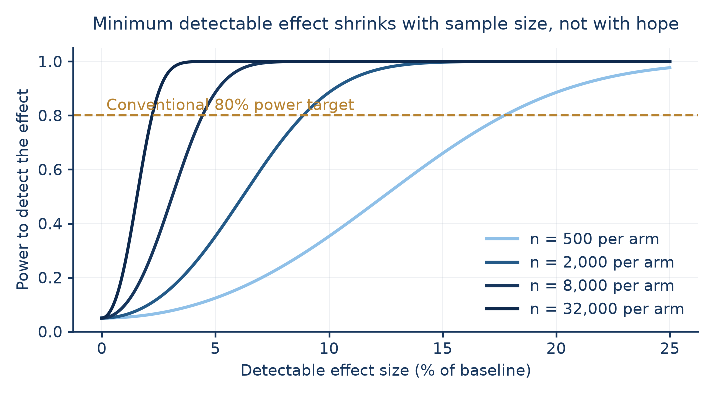
Minimum detectable effect
A negative result is worthless without an MDE.
"No effect detected at 500 changes per arm" ≈ "no effect > 15% detectable"
Same result at 32,000 per arm ≈ "no effect > 2% detectable"
Power analyses belong in the pre-registration, not the discussion.
Segment 3 (20 min)
Open companion/notebooks/05-power-and-mde.py.
Type in your outcome σ and the effect you actually care about. What’s the required per-arm sample? How long would it take at your team’s throughput?
Report back: one experiment you thought was possible that isn’t at your scale.
Sequential testing
Engineering experiments run continuously. Teams peek.
Repeated naive tests at α = 0.05 inflate false positives fast:
1 look: 5%
5 looks: ~14%
10 looks: ~19%
Solution: group-sequential boundaries that spend α over planned looks.
O’Brien-Fleming boundary
At K planned looks:
Very strict early. Approaches conventional α by the final look.
Look 1 of 5: reject if \(|z| > 4.56\)
Look 3 of 5: reject if \(|z| > 2.63\)
Look 5 of 5: reject if \(|z| > 2.04\)
Segment 4 (20 min)
Open companion/notebooks/12-sequential-testing.py.
Simulate 5,000 runs of a null-effect experiment. Compare naive repeated α = 0.05 versus O’Brien-Fleming.
Report back: the difference in type-I error you observed.
Don’ts, worth memorising
Don’t rely on before-after alone. Bring a control group or a plausible counterfactual.
Don’t launch without a pre-analysis plan and pre-declared MDE.
Don’t peek without a boundary.
Don’t confuse ITT and CACE in the executive summary.
Don’t retire a Class 2+ metric without a versioned replacement.
Wrap-up
Draw a DAG before you launch
Pick the estimand that matches the decision
Compute MDE before collecting data
Peek only under a boundary
Read: Chapter 6 of Engineering Intelligence.
Run: companion/notebooks/04, 05, 12.
Iterate: one experiment per quarter on a decision that actually matters.
References: [hernan2020], [imbens2015], [angrist2009].