"Counting" sounds like the first thing you learned in mathematics. One, two, three. But try these:

You could, in principle, list every case and count. In practice, the lists contain thousands or millions of items, and the classic mistakes are counting something twice or missing a whole family of cases. Combinatorics is the branch of mathematics that counts without listing. Its tools let you reduce "how many?" to a short calculation that you can trust.

Every counting technique in this chapter does one of three things:

If you remember those three moves, the formulas follow.

A café offers 3 mains (pasta, curry, salad) and 2 drinks (tea, water). How many different main-plus-drink meals are there? And if instead you may order either a main or one of 4 desserts (but not both), how many single-item orders are there?

For the meal, imagine making the choice in two stages. First pick a main: 3 branches. From each main, pick a drink: 2 branches. Every complete path from the root to a leaf is one meal, so the number of meals is the number of leaves.

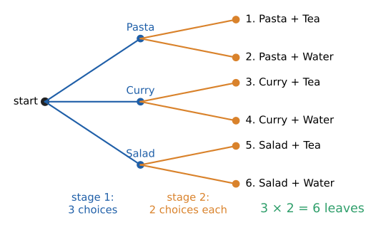
Each of the 3 first-stage branches sprouts the same number (2) of second-stage branches, so there are \(3 \times 2 = 6\) leaves. That is the product rule.

For "a main or a dessert", there is no sequence of stages, just two disjoint pools of options. You pick from one pool or the other, so there are \(3 + 4 = 7\) options. That is the sum rule.

The product rule is really the area of a rectangle. Lay the first-stage options along one side of a grid and the second-stage options along the other. Each cell is one pair, so there are \(m\) rows of \(n\) cells: \(mn\) cells. In set language, the outcomes form the Cartesian product \(A \times B = \{(a, b) : a \in A,\ b \in B\}\), and \(|A \times B| = |A|\,|B|\). With more stages you get a box, or a higher-dimensional box, and the count is still the product of the side lengths.

The important fine print is "for each". The second stage need not offer the same options each time, only the same number of options. When you choose a gold, then a silver medallist from 8 runners, the silver choices depend on who won gold, but there are always 7 of them.

A (hypothetical) number plate is 3 letters followed by 4 digits, such as KTX 3071. How many plates are possible? How many if no letter and no digit may repeat? Try it: Count number plates in stages.

Stages: letter 1, letter 2, letter 3, digit 1, …, digit 4. Seven stages.

With repetition allowed, every letter stage has 26 options and every digit stage has 10:

Without repetition, each stage loses one option for each earlier choice of the same kind: Try it: Plates without repeats.

How many positive integers less than 1000 have digits that are all odd?

Split by number of digits (disjoint cases, so add):

How many 4-digit PINs (0000 to 9999) contain at least one repeated digit? "At least one" questions split into many messy cases (exactly one pair, two pairs, a triple …). Instead, count what you don’t want and subtract from the total: Try it: PINs with no repeated digit.

Almost half of all PINs repeat a digit. Counting the complement is the single most useful trick in elementary counting, and it is exactly the move behind the birthday paradox later in this chapter.

Biology: why the genetic code uses triplets. DNA has 4 bases and must encode 20 amino acids. Words of 2 bases give only \(4^2 = 16\) possibilities, too few; words of 3 give \(4^3 = 64\), enough with room to spare. The product rule predicts the three-letter codon, and the spare capacity shows up as redundancy: most amino acids have several codons.

Engineering: test matrices. A web app that must work on 3 browsers, 4 operating systems and 2 languages has \(3 \times 4 \times 2 = 24\) configurations. Add 5 screen sizes and it is 120. Product-rule growth is why testers use pairwise testing, which covers every pair of settings with far fewer runs.

Everyday. A combination bike lock with 4 dials of 10 digits has \(10^4 = 10\,000\) settings; at one try every 2 seconds, trying them all takes under 6 hours. A 3-dial lock (1,000 settings) falls in about half an hour.

Eight runners contest a race. In how many ways can gold, silver and bronze be awarded? In how many ways can all eight finish, in order?

Fill the podium one step at a time. Any of the 8 runners can win gold. Whoever wins, 7 remain for silver, then 6 for bronze. The product rule gives \(8 \times 7 \times 6 = 336\). For a complete finishing order, keep going all the way down: \(8 \times 7 \times 6 \times 5 \times 4 \times 3 \times 2 \times 1\).

There are \(r\) stages. Stage 1 has \(n\) options. Each earlier stage has used up one object, so stage \(i\) has \(n - (i-1)\) options. The last stage, stage \(r\), has \(n - r + 1\). By the product rule,

To see the factorial form, multiply and divide by the "missing tail" \((n-r)!\):

The product form is better for hand calculation (\(P(8, 3) = 8 \cdot 7 \cdot 6\) is immediate, while \(8!/5!\) invites you to compute two large numbers and divide). The factorial form is better for algebra.

With \(r = n\), the formula says \(P(n, n) = n!/0!\). But \(P(n, n)\) is the number of orderings of all \(n\) objects, which is \(n!\). So \(0!\) has to be \(1\) for the formula to work. There is also a direct reason: there is exactly one way to arrange nothing (the empty arrangement). And the recursion \(n! = n \cdot (n-1)!\) at \(n = 1\) gives \(1 = 1 \cdot 0!\). Three different arguments, one answer: this is a definition chosen because it makes everything consistent, not an arbitrary rule.

Podium. \(P(8, 3) = 8 \times 7 \times 6 = 336\).

Full finishing order. \(8! = 40\,320\).

Seating with a constraint. Five people, including Ann and Bob, sit in a row. In how many arrangements are Ann and Bob next to each other?

Glue Ann and Bob into a single block. Now arrange 4 units (the block and three others), then arrange the two people inside the block:

As a check, the arrangements where they are not adjacent number \(5! - 48 = 120 - 48 = 72\).

Round table. In how many ways can 5 people sit round a circular table, if only who sits next to whom matters (rotations are the same seating)? Each circular seating corresponds to 5 different linear ones (start reading at any of the 5 seats), so the count is \(5!/5 = 4! = 24\). In general, \((n-1)!\) circular arrangements. This is your first glimpse of "count something easier, then divide out the over-count". Try it: Round-table seatings counted five times.

Sport. With 8 sprinters in a final, the number of possible podiums (gold, silver, bronze) is \(P(8, 3) = 8 \cdot 7 \cdot 6 = 336\). Order matters, so it is a permutation; the number of possible sets of medallists is only \(336 / 3! = 56\).

Logistics. A delivery driver with 10 drops can visit them in \(10! = 3\,628\,800\) orders. With 20 drops it is about \(2.4 \times 10^{18}\), which is why route planners use heuristics instead of checking every order (the travelling salesman problem, Chapter 25).

History of cryptography. The German Army’s Enigma machine placed 3 of its 5 rotors into 3 slots, and order mattered: \(P(5, 3) = 60\) wheel orders. Each of the 60 had to be tested separately, which is one reason the Bletchley Park codebreakers built banks of electromechanical "bombes" to run in parallel.

A club of 10 people must choose a committee of 3. How many different committees are possible?

You already know how to count ordered choices: \(P(10, 3) = 10 \cdot 9 \cdot 8 = 720\). But a committee is a set of people; {Ann, Bob, Cat} is the same committee however you list them. Each committee shows up in the ordered count once for each of its orderings, and three people can be ordered in \(3! = 6\) ways: Try it: Each committee counted 3! times.

Every committee is counted exactly 6 times, so the number of committees is \(720 / 6 = 120\).

Here is the derivation made precise. Consider all ordered selections of \(r\) objects from \(n\). Build each one in two stages:

Every ordered selection arises exactly once this way, so by the product rule

This is the division principle: if a count treats every object you care about exactly \(k\) times, divide by \(k\).

For hand calculation, use the cancelled form: \(\binom{n}{r} = \dfrac{n (n-1) \cdots (n-r+1)}{r!}\), with \(r\) factors on top and \(r!\) below.

Choosing the 3 people who are on the committee is the same as choosing the 7 who are not. So

The formula confirms it (swap \(r\) and \(n-r\) in the denominator), but the counting argument says why. It also saves work: \(\binom{100}{98} = \binom{100}{2} = \dfrac{100 \cdot 99}{2} = 4950\).

From 10 people (4 women and 6 men), how many 4-person committees have exactly 2 women?

Stage 1, choose the women; stage 2, choose the men. These are independent, so multiply:

How many have at least one woman? Use the complement:

Choose a 3-person committee from 10 and name one of the three as chair. Two methods: Try it: Committee with a chair, both ways.

Both agree, which is the point. When you can count the same set two ways, you have not just a check but an identity: \(3\binom{10}{3} = 10\binom{9}{2}\), and in general \(r\binom{n}{r} = n\binom{n-1}{r-1}\). Proofs of this kind, called double counting or combinatorial proofs, are the subject’s favourite technique, and you will use one next for Pascal’s rule.

Try it: See the 336 over-count.

Sport. A 20-team league in which every pair of teams meets twice (home and away) plays \(2\binom{20}{2} = 380\) matches, which is exactly the length of an English Premier League season.

Engineering: links in a network. Connecting every pair of 50 offices directly needs \(\binom{50}{2} = 1225\) links; routing everything through one hub needs 49. That quadratic-versus-linear gap is why telephone exchanges, Ethernet switches and airline hubs exist.

Science: screening combinations. A lab with 20 candidate drugs that wants to test every pair needs \(\binom{20}{2} = 190\) experiments; every triple needs \(\binom{20}{3} = 1140\). Counting first tells you whether an exhaustive screen is affordable or whether you need a statistical design that samples combinations.

Everyday. Choosing 3 pizza toppings from 12 gives \(\binom{12}{3} = 220\) different pizzas, and the menu that boasts "over 200 combinations" is quoting exactly this number.

Computing \(\binom{n}{r}\) from factorials is fine for a calculator, but it hides a beautiful structure. Is there a way to build all the binomial coefficients from simpler ones, without any multiplication or division?

Write \(\binom{n}{0}, \binom{n}{1}, \ldots, \binom{n}{n}\) as row \(n\) of a triangle, rows centred:

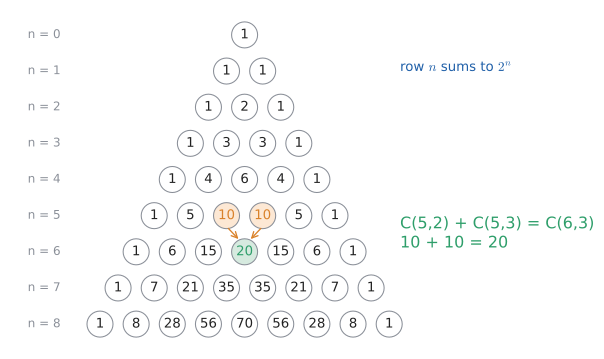
Each row begins and ends with 1, and every interior entry is the sum of the two diagonally above it. In symbols, that is Pascal’s rule. Try it: Explore Pascal’s triangle.

You could prove this by adding fractions of factorials. The counting proof is shorter and tells you why.

Proof. Count the \(r\)-element subsets of a set of \(n\) people, one of whom is called Zoe. The left side, \(\binom{n}{r}\), counts all of them directly. Now sort the subsets into two disjoint cases:

Every subset is in exactly one case, so by the sum rule the total is \(\binom{n-1}{r-1} + \binom{n-1}{r}\). Both sides count the same set, so they are equal. \(\blacksquare\)

This "single out one element and ask whether it’s in" move is also the recursion behind many algorithms (the 0/1 knapsack dynamic programme makes exactly this decision for each item).

For example, \(\binom{8}{3}\): \(c = 1 \cdot 6/1 = 6\), then \(6 \cdot 7/2 = 21\), then \(21 \cdot 8/3 = 56\). The intermediate values 6, 21, 56 are themselves binomial coefficients (\(\binom{6}{1}, \binom{7}{2}, \binom{8}{3}\)). If instead you need a whole table, build Pascal’s triangle by addition, which is what a dynamic-programming solution does.

Try it: Sierpiński in 64 rows.

Expand \((x + y)^5\) without multiplying out five brackets by hand. More generally, what is the coefficient of \(x^3 y^2\) in \((x+y)^5\), and why are binomial coefficients called binomial?

Write \((x+y)^3 = (x + y)(x + y)(x + y)\). Fully expanding means: from each of the three brackets pick either \(x\) or \(y\), multiply your three picks, and add up the results over all \(2^3 = 8\) ways of picking:

Try it: Pick x or y, visually.

The term \(x^2 y\) appears once for each way of choosing which one bracket supplies the \(y\): \(\binom{3}{1} = 3\) ways (xxy, xyx, yxx). So

The coefficients 1, 3, 3, 1 are row 3 of Pascal’s triangle. That is why they’re called binomial coefficients: they are the coefficients in the expansion of a power of a binomial (a two-term expression).

For any numbers \(x, y\) and non-negative integer \(n\),

Why. Each term of the expansion comes from choosing \(x\) or \(y\) from each of the \(n\) brackets. A choice that takes \(y\) from exactly \(k\) brackets (and so \(x\) from the other \(n-k\)) contributes \(x^{n-k} y^k\). The number of such choices is the number of ways to pick which \(k\) brackets supply \(y\), namely \(\binom{n}{k}\). Collect like terms and you get the theorem. (A proof by induction using Pascal’s rule also works; see Chapter 22. The counting proof is the one that explains it.)

Here \(a = x\), \(b = 2\), \(n = 4\); row 4 is 1, 4, 6, 4, 1. Try it: Expand (x + 2)⁴.

Check by substituting \(x = 1\): the left side is \(3^4 = 81\); the right side is \(1 + 8 + 24 + 32 + 16 = 81\). Substituting a convenient value is a quick, reliable test of any expansion.

Find the coefficient of \(x^3\) in \((2x - 1)^5\). You do not need the whole expansion. Here \(a = 2x\), \(b = -1\), \(n = 5\). A term has the form \(\binom{5}{k}(2x)^{5-k}(-1)^k\), which contains \(x^{5-k}\). For \(x^3\) you need \(5 - k = 3\), so \(k = 2\): Try it: Find the x³ coefficient.

The coefficient is \(80\).

Genetics: how likely is "exactly one"? Two parents who both carry a recessive gene each pass it on with probability \(\tfrac12\), so each child is affected with probability \(\tfrac14\). In a family of 4 children, the chance that exactly one is affected is one term of the binomial expansion of \((\tfrac14 + \tfrac34)^4\): Try it: Exactly one of four children.

The coefficient 4 counts which child it is; the powers give the probability of one particular pattern. Chapter 30 turns this into the binomial distribution.

Finance and physics: quick approximations. The truncated expansion above, \((1 + y)^n \approx 1 + ny\), is how people estimate small compound changes in their heads (2% a year for 5 years is roughly 10%; the exact figure is 10.4%), and how physicists simplify formulas such as \((1 - v^2/c^2)^{-1/2} \approx 1 + \tfrac12 v^2/c^2\) at everyday speeds (the binomial series for non-integer powers, Chapter 14).

How many 4-letter "words" (any strings, not necessarily English) use the letters A–Z? How many distinct rearrangements are there of the letters of MISSISSIPPI?

When repetition is allowed and order matters, each of the \(r\) positions independently has \(n\) options:

So there are \(26^4 = 456\,976\) four-letter strings, \(10^4\) four-digit PINs, and \(2^n\) bit strings of length \(n\). This is the count behind every keyspace calculation in security.

MISSISSIPPI has 11 letters, but they are not all distinct: M once, I four times, S four times, P twice. If the letters were all different (label them \(I_1, I_2, I_3, I_4\) and so on), there would be \(11!\) arrangements. But swapping the labelled I’s among themselves gives the same word; each word is counted \(4!\) times on account of the I’s, and likewise \(4!\) for the S’s and \(2!\) for the P’s. Divide out each over-count: Try it: Step through MISSISSIPPI anagrams.

Another way to see it. Place the letters into 11 slots in stages: choose 1 slot for M, then 4 of the remaining 10 for the I’s, then 4 of the remaining 6 for the S’s, and the last 2 go to the P’s:

Same answer, by a method that never divides. Both are worth having: the first is faster to write, the second is easier to justify step by step.

Grid paths. How many shortest routes are there on a city grid from one corner to a point 5 blocks east and 3 blocks north? Every shortest route is a string of 5 E’s and 3 N’s in some order, so the count is \(\binom{8}{3} = 56\). Recognising a problem as "arrangements of a multiset" in disguise is a recurring skill. Try it: Walk the 56 grid routes.

An ice-cream shop has 3 flavours: vanilla, chocolate and mint. You order a tub of 7 scoops. Scoops of the same flavour are identical, and only how many of each flavour you get matters. How many different tubs are there?

In algebraic form: how many solutions are there to

Draw each scoop as a star \(\star\) and separate the flavours with 2 bars:

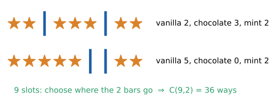
Stars before the first bar are vanilla, between the bars chocolate, after the second bar mint. Two bars together (||*) means zero chocolate. Every tub gives exactly one such string, and every string of 7 stars and 2 bars gives exactly one tub. So count the strings: 9 positions, choose which 2 hold bars: \(\binom{9}{2} = 36\). Try it: Drag the stars and bars.

Distributing \(n\) identical objects into \(k\) distinct boxes (empty boxes allowed) uses \(n\) stars and \(k - 1\) bars, so

Equivalently, this is the number of multisets of size \(n\) drawn from \(k\) types: unordered selection with repetition. That fills the last cell of the order/repetition table.

How many tubs of 7 scoops have at least one scoop of each flavour (\(x_i \ge 1\))? Try it: At least one of each.

Hand out one scoop of each flavour first. That leaves 4 scoops to distribute freely among 3 flavours: \(y_1 + y_2 + y_3 = 4\) with \(y_i = x_i - 1 \ge 0\):

Alternatively, think of the 7 stars in a row with 6 gaps between them; placing 2 bars in 2 different gaps (no empty flavour) is \(\binom{6}{2} = 15\).

A shop sells 5 kinds of doughnut. How many different boxes of 12 can you buy? Here \(n = 12\) objects into \(k = 5\) kinds: Try it: List the 1820 doughnut boxes.

Physics: counting microstates. In the simplest model of a solid (Einstein’s), energy comes in identical packets, quanta, shared among atomic oscillators. The number of ways to share \(q\) quanta among \(N\) oscillators is a stars-and-bars count, \(\binom{q + N - 1}{q}\). Three quanta among three oscillators: \(\binom{5}{3} = 10\) microstates (3-0-0 in 3 ways, 2-1-0 in 6 ways, 1-1-1 in 1 way). Statistical mechanics defines entropy from exactly this count, and it is why heat flows from hot to cold: that direction has overwhelmingly more microstates.

Everyday. Splitting $10 of pocket money, in whole dollars, between saving, spending and giving: \(\binom{12}{2} = 66\) possible plans. Allocating 6 identical seats among 3 parties: \(\binom{8}{2} = 28\) possible results.

Of the integers from 1 to 1000, how many are divisible by 2, by 3 or by 5?

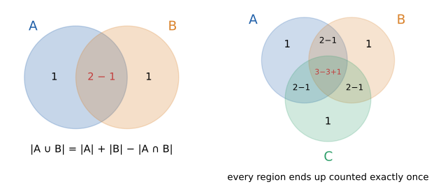
For two sets, adding \(|A| + |B|\) counts the overlap twice, so subtract it once:

For three sets, adding the three sizes counts each two-way overlap twice and the triple overlap three times. Subtracting the three pairwise intersections fixes the two-way regions, but now the triple region has been added 3 times and subtracted 3 times, so it isn’t counted at all. Add it back once:

For \(k\) sets the pattern continues: add the single sets, subtract all pairwise intersections, add all triple intersections, subtract quadruples, and so on, with alternating signs. Why does every element end up counted exactly once? Take an element that lies in exactly \(m \ge 1\) of the sets. It is counted \(\binom{m}{1}\) times in the singles, \(\binom{m}{2}\) times in the pairs, and so on, so its total count is

using the alternating-sum identity from the binomial theorem (put \(x = 1, y = -1\) in \((x + y)^m\)). The two big ideas of the chapter meet here.

Let \(A_2\), \(A_3\), \(A_5\) be the multiples of 2, 3, 5 in \(\{1, \ldots, 1000\}\). The number of multiples of \(d\) up to \(N\) is \(\lfloor N/d \rfloor\) (the floor, or integer part, of \(N/d\)). A number divisible by both 2 and 3 is divisible by 6, and so on (because 2, 3, 5 are pairwise coprime; see Chapter 23). Try it: Multiples of 2, 3, 5, counted.

So 734 numbers are divisible by at least one of 2, 3, 5, and \(1000 - 734 = 266\) are divisible by none. A one-line brute-force check agrees:

Try it: Derangements racing to 1/e; Count the 9 derangements.

Everyday: who takes which class. A school has 120 students; 50 take French, 40 Spanish and 30 German; 15 take French and Spanish, 10 French and German, 8 Spanish and German, and 3 take all three. Then \(50 + 40 + 30 - 15 - 10 - 8 + 3 = 90\) take at least one language, so 30 take none. Checking region by region (28 French only, 20 Spanish only, 15 German only, 12, 7 and 5 in exactly two, 3 in all) gives the same 90.

Security: password policies. How many 8-character passwords over the 62 letters and digits contain at least one digit, one lowercase and one uppercase letter? Count the complement with inclusion–exclusion. Passwords missing digits number \(52^8\); missing lowercase, \(36^8\); missing uppercase, \(36^8\). Missing two classes: \(26^8 + 26^8 + 10^8\). Missing all three: 0. So the policy allows Try it: Password policy by inclusion–exclusion.

about 73% of the \(2.18 \times 10^{14}\) unrestricted strings. Composition rules shrink the keyspace slightly; it is length that grows it.

Science: overlapping risk factors. Epidemiologists use the same bookkeeping on patient records: the number with any of several conditions is the sum of the counts, minus the pairwise overlaps, plus the triple overlap. Forgetting the overlaps overstates prevalence, which is exactly the double counting the formula corrects.

Some counting questions ask not "how many?" but "must something happen?" In a drawer of black, blue and grey socks, how many must you pull out in the dark to be sure of a matching pair? In any group of 367 people, must two share a birthday?

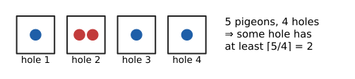
If more than \(k\) objects are placed into \(k\) boxes, some box contains at least two objects.

Proof. If every box held at most one object, there would be at most \(k\) objects. \(\blacksquare\) (A one-line proof by contradiction; see Chapter 22.)

Generalised form. If \(N\) objects go into \(k\) boxes, some box contains at least \(\lceil N/k \rceil\) objects. (Otherwise every box holds at most \(\lceil N/k \rceil - 1 < N/k\) objects, for fewer than \(k \cdot N/k = N\) in total.)

The principle is almost embarrassingly obvious. Its power lies in choosing the pigeons and holes cleverly.

Most "choose \(r\) things from \(n\) types" problems are settled by two yes/no questions:

Notice how the table is held together by the earlier ideas. Moving down the left column, \(n^r\) becomes \(n(n-1)\cdots\) because each stage loses an option. Moving right along the bottom row, you divide by the \(r!\) orderings. The top-right cell is stars and bars.

From the digits 1–5, form a selection of 3.

As a sanity check, the counts must satisfy \(10 \le 35 \le 125\) and \(10 \le 60 \le 125\), since allowing more freedom never reduces the count.

A 6/49 lottery draws 6 distinct numbers from 1–49; order doesn’t matter. The number of tickets is

One ticket wins the jackpot with probability about 1 in 14 million. US Powerball draws 5 white balls from 69 and 1 red ball from 26: \(\binom{69}{5} \times 26 = 11\,238\,513 \times 26 = 292\,201\,338\) combinations, so the jackpot odds are 1 in about 292 million. A second prize such as "match exactly 5 of 6" in the 6/49 game is a product of combinations: choose 5 of the 6 winning numbers and 1 of the 43 losing numbers, \(\binom{6}{5}\binom{43}{1} = 6 \times 43 = 258\) tickets.

A password of length \(L\) over an alphabet of \(a\) symbols has \(a^L\) possibilities (ordered, repetition allowed). Length matters far more than alphabet size, because length is the exponent:

Going from 26 to 62 symbols at length 8 multiplies the space by about 1000. Going from length 8 to 12 at 62 symbols multiplies it by \(62^4 \approx 1.5 \times 10^7\). The CS section below turns these counts into cracking times.

A five-card hand from a 52-card deck is an unordered selection without repetition: \(\binom{52}{5} = 2\,598\,960\) hands. Counting particular hands is a perfect exercise in staged construction. The rule: build the hand by deciding the ranks, then the suits, making sure each hand is built once.

Four of a kind (e.g. four 7s and a king). Choose the rank of the four: 13. All four suits are forced: \(\binom{4}{4} = 1\). Choose the fifth card from the 48 others: 48.

Full house (three of one rank, two of another). Choose the rank of the triple, then its suits; choose a different rank for the pair, then its suits:

Here the two ranks are chosen in order (13 then 12) because their roles differ: "three kings and two 7s" is a different hand from "three 7s and two kings".

Two pair (two of one rank, two of another, and a fifth card of a third rank). Now the two pair ranks play the same role, so choose them as a set:

(The fifth card can be any of the \(52 - 8 = 44\) cards not of either pair rank.) If you’d used \(13 \times 12\) for the pair ranks, you’d have built each hand twice and got 247,104.

One pair. Choose the pair rank and suits, then 3 different other ranks (as a set) and a suit for each:

Flush (all five the same suit, excluding straight flushes): \(4 \times \binom{13}{5} - 40 = 4 \times 1287 - 40 = 5108\), where 40 is the number of straight flushes (4 suits × 10 possible starting ranks, ace low to ten high).

Dividing by 2,598,960 gives the probabilities: a full house is about 0.144 %, four of a kind about 0.024 %. Rarer hands beat commoner ones, which is exactly the ranking used in the game. That is not a coincidence: the ranking was settled by counting.

An attacker who has stolen a database of password hashes can guess offline as fast as their hardware allows. For a fast, unsalted hash, a single modern GPU rig can try on the order of \(10^{10}\) guesses per second. The expected time to search the whole keyspace is (keyspace) / (rate); on average the right password is found halfway through. Try it: Password keyspace calculator.

Try it: Time to crack 12 characters.

Two lessons follow. First, exponential growth in length beats everything: every extra character multiplies the work by the alphabet size. Second, these are upper bounds on safety: human-chosen passwords are not uniformly random, so attackers try dictionaries and patterns first, and the effective keyspace is far smaller. That’s why systems use deliberately slow, salted hash functions (bcrypt, scrypt, Argon2) to cut the guess rate by many orders of magnitude, and why a passphrase of 5 random dictionary words (from a list of 7776, as in Diceware) gives \(7776^5 \approx 2.8 \times 10^{19}\) possibilities while staying memorable.

Security engineers express keyspaces in bits: a keyspace of size \(N\) has \(\log_2 N\) bits of entropy (if every key is equally likely). \(62^{12} \approx 2^{71.5}\), so a random 12-character alphanumeric password is a 71-bit secret. A 128-bit AES key gives \(2^{128} \approx 3.4 \times 10^{38}\) keys.

A set of \(n\) elements has \(2^n\) subsets: for each element, "in" or "out". There’s a perfect correspondence between subsets and \(n\)-bit binary numbers (bit \(i\) is 1 if element \(i\) is in), which gives the simplest way to enumerate them:

Any algorithm that tries every subset (the brute-force approach to subset-sum, knapsack, feature selection or set cover) does at least \(2^n\) units of work, and any algorithm that tries every ordering (brute-force travelling salesman) does \(n!\).

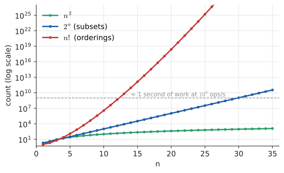
At a billion operations a second, \(2^{30} \approx 10^9\) subsets take a second, \(2^{40}\) take about 18 minutes, \(2^{50}\) take 13 days, and \(2^{60}\) take 36 years. \(20! \approx 2.4 \times 10^{18}\) orderings take 77 years. Faster hardware barely helps: a computer 1000 times faster raises the feasible \(n\) for a \(2^n\) algorithm by only about 10. This is why the distinction between polynomial and exponential running time is the central dividing line of complexity theory, and why, for problems like these, practical algorithms use pruning, dynamic programming, or approximation instead of enumeration.

Sometimes you really do need to visit every arrangement: testing all orderings of a small set of operations for race conditions, solving a puzzle exhaustively, or generating test cases. Two standard algorithms do this.

Next permutation (lexicographic order). Given an arrangement, produce the next one in dictionary order. This is what C++'s std::next_permutation does, and it handles repeated items gracefully (it produces each distinct arrangement once).

The idea: to get the next larger arrangement, change as far to the right as possible. Find the longest suffix that is already in descending order (it is the largest possible arrangement of those items, so it can’t be increased by itself). The element just before it, the pivot, must increase, by the smallest possible amount, and then the suffix must be reset to its smallest arrangement (ascending).

Worked trace on \((1, 3, 5, 4, 2)\): Try it: Step through next permutation.

Check: among arrangements starting \(1, 3, \ldots\), \((1, 3, 5, 4, 2)\) is the largest; the next must start \(1, 4\), followed by the remaining \(\{2, 3, 5\}\) in ascending order. That’s \((1, 4, 2, 3, 5)\).

Try it: All permutations in order; Permutations with repeated items.

The last line lists \(3!/2! = 3\) arrangements, the multinomial count for \(\{1, 1, 2\}\), not \(3! = 6\).

Backtracking. The other approach builds arrangements position by position, mirroring the product rule’s stages: choose an unused item for the next position, recurse, then undo the choice and try the next item. It is the template for a huge family of search algorithms (sudoku, N-queens, constraint solvers), because you can prune: abandon a partial arrangement as soon as it violates a constraint, skipping every completion of it at once. Try it: Backtracking with pruning (4 queens).

Try it: Watch the recursion tree.

Choosing between them. In production Python, just use itertools.permutations; it is implemented in C. Use next-permutation when you need to step through arrangements one at a time with constant extra memory, or when items repeat and you want each distinct arrangement once. Use backtracking when you want to prune, which is almost always the case in real search problems.

The recursion tree of the backtracking algorithm is the product-rule tree diagram from Section 24.2: \(n\) branches at the root, \(n - 1\) at the next level, and so on, with \(n!\) leaves.

How many people must be in a room for there to be a better than even chance that two share a birthday? The pigeonhole principle says 367 people make it certain; the surprise is how few make it likely.

Count the complement. Assume 365 equally likely birthdays (ignoring 29 February). The number of ways \(n\) people can have all different birthdays is \(P(365, n)\) (ordered, no repetition) out of \(365^n\) total assignments, so

(The symbol \(\prod\) is the product version of \(\sum\): multiply the terms instead of adding them.) The probability language is developed properly in Chapter 29; here you need only "favourable over total", with every assignment equally likely.

Try it: Simulate the birthday problem.

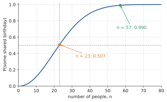
Why so few? Because what matters is the number of pairs, not the number of people. 23 people form \(\binom{23}{2} = 253\) pairs, and each pair has a 1-in-365 chance of matching. Using \(1 - x \approx e^{-x}\) for small \(x\),

where \(N\) is the number of possible values. Setting this to \(\tfrac12\) and solving gives \(n \approx \sqrt{2 \ln 2 \cdot N} \approx 1.18\sqrt{N}\). For \(N = 365\), that’s about 22.5. The rule of thumb: collisions become likely after about \(\sqrt{N}\) random items.

Hash collisions. Replace birthdays with hash values. A hash table, a content-addressed store, or a database of short IDs with \(N\) possible values will see its first collision after about \(\sqrt{N}\) items, not \(N\). A 32-bit hash (\(N \approx 4.3 \times 10^9\)) has a 50 % chance of a collision after only about 77,000 items, which is why 32-bit checksums are useless as unique identifiers for large collections. A 64-bit hash reaches 50 % at about 5 billion items. Cryptographic hashes use 256 bits so that the "birthday bound" \(2^{128}\) is far beyond any attacker; a hash with \(b\)-bit output offers only about \(b/2\) bits of collision resistance. The same arithmetic tells you how long random UUIDs (122 random bits) can be generated before a duplicate is plausible: around \(2^{61} \approx 2.3 \times 10^{18}\).