Volume 1: Foundations to Precalculus · Part IV: Functions, Trigonometry, and Precalculus
Chapter 12. Exponentials and Logarithms
Some quantities grow by adding the same amount each step. Others grow by multiplying by the same factor each step, and those behave in a completely different way. This chapter is about the second kind. It covers exponential functions, the special number \(e\) that comes out of compound interest, and the logarithm, which answers the question "what power?". Logarithms turn multiplication into addition, which is why they show up in decibels, earthquake magnitudes, binary search, information theory and the numerical guts of machine learning.
Why it matters: savings, loans, inflation, epidemics, radioactive dating, drug doses, cooling coffee, network retry timers and the cost of brute-forcing a password all follow the same multiply-by-a-constant rule. Misjudging exponential growth is one of the most expensive mistakes people make with money and with forecasts, and logarithms are the tool that tames it.
12.1. Growth by multiplication
12.1.1. The problem
Take a sheet of paper 0.1 mm thick and fold it in half. It is now 0.2 mm thick. Fold it again: 0.4 mm. How many folds would it take for the stack to reach the Moon, about 384,400 km away?
Most people guess thousands, or millions. The answer is 42.
Here is a second puzzle that is really the same one. A rumour starts with one person. Every hour, everyone who knows it tells one new person. After one day (24 hours), how many people know?
After a day and a half, more people than live on Earth would "know", which is obviously impossible. Something has to give. We come back to that in Section 12.7.
What these puzzles share is a quantity that gets multiplied by the same factor at every step. That is the defining feature of exponential behaviour, and human intuition is very bad at it.
12.1.2. Intuition: constant difference versus constant ratio
Compare two savings plans, each starting at $100:
-
Plan L adds $10 every year.
-
Plan E adds 10% of the current balance every year, so the balance is multiplied by 1.1.
| Year | Plan L | L: change | Plan E | E: ratio |
|---|---|---|---|---|
0 |
100 |
— |
100.00 |
— |
1 |
110 |
+10 |
110.00 |
×1.1 |
2 |
120 |
+10 |
121.00 |
×1.1 |
3 |
130 |
+10 |
133.10 |
×1.1 |
10 |
200 |
+10 each |
259.37 |
×1.1 each |
50 |
600 |
+10 each |
11,739.09 |
×1.1 each |
In the early years the two plans are almost the same. Over time the multiplying plan leaves the adding plan far behind. The rule of thumb:
-
Linear growth: equal steps in input give equal differences in output. The graph is a straight line (Chapter 5).
-
Exponential growth: equal steps in input give equal ratios in output. The graph bends upward faster and faster.
You can recognise exponential data in a table by dividing each value by the one before. If the ratios are all (roughly) the same, the data is exponential.
12.1.3. Vocabulary and notation
|
Exponential function
An exponential function has the variable in the exponent:
\[f(x) = a \cdot b^{x}, \qquad b > 0,\ b \neq 1.\]
Compare it with a power function such as \(x^2\), where the variable is in the base. \(x^2\) and \(2^x\) are very different functions. |
|
Growth rate, decay rate
If something grows by a percentage \(r\) per step (written as a decimal, so 5% means \(r = 0.05\)), its growth factor is \(b = 1 + r\). If it decays (shrinks) by \(r\) per step, then \(b = 1 - r\).
\(r\) is the growth rate (or decay rate). \(b\) is the growth factor. Don’t mix the two up: a 5% rate is a factor of 1.05. |
|
Doubling time and half-life
The doubling time of an exponentially growing quantity is the time it takes to double. The half-life of a decaying quantity is the time it takes to halve. For an exponential process these are constant: going from 100 to 200 takes exactly as long as going from 1,000 to 2,000. With a half-life \(T\), the amount after time \(t\) is
\[N(t) = N_0 \left(\tfrac{1}{2}\right)^{t/T}.\]
Here \(N_0\) ("N nought") is the starting amount and \(t/T\) counts how many half-lives have gone by. |
12.1.4. Why the model works
If a quantity is multiplied by \(b\) each step and starts at \(a\), then
So "multiply by \(b\) every step" turns into "raise \(b\) to the number of steps". The exponent counts the multiplications.
Now look again at the folding puzzle. Thickness after \(n\) folds is \(0.1 \times 2^{n}\) mm. For \(n = 42\):
which is more than the 384,400 km to the Moon. (41 folds gives about 219,900 km, which is not enough.) Doubling 42 times multiplies by more than four trillion.
From Chapter 3 you know that \(b^x\) makes sense for any real \(x\), not only whole numbers: \(b^{1/2} = \sqrt{b}\), \(b^{-1} = 1/b\), and irrational exponents are filled in by continuity. So \(f(x) = a b^x\) is defined on the whole real line and gives a smooth curve.
12.1.5. The graph of \(b^x\)
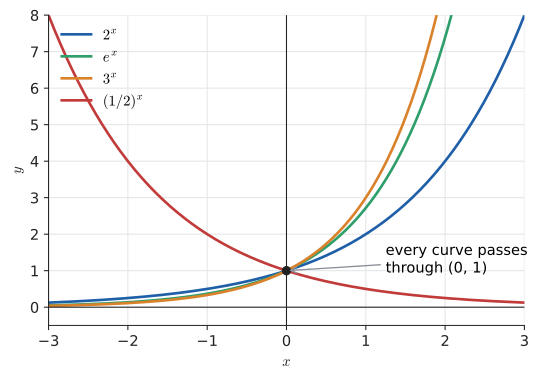
Every graph of \(y = b^x\) with \(b > 0\), \(b \ne 1\) shares these features:
-
Domain: all real numbers. You can raise a positive base to any power.
-
Range: \(y > 0\). A positive base raised to any power is positive, so the graph never touches or crosses the \(x\)-axis.
-
y-intercept: \((0, 1)\), because \(b^0 = 1\).
-
Horizontal asymptote: the \(x\)-axis, \(y = 0\). For \(b > 1\) the curve gets arbitrarily close to it as \(x \to -\infty\). For \(b < 1\) that happens as \(x \to +\infty\).
-
One-to-one: each output comes from exactly one input. That means the function has an inverse, and the inverse is the logarithm.
-
\((1/b)^x = b^{-x}\), so the graph of \((1/2)^x\) is the graph of \(2^x\) reflected in the \(y\)-axis.
|
Asymptote
An asymptote is a line that a curve approaches more and more closely without reaching it (at least far out). \(y = 0\) is a horizontal asymptote of \(y = 2^x\): as \(x\) becomes very negative, \(2^x\) gets as close to 0 as you like but stays positive. |
12.1.6. Worked example: radioactive decay
Carbon-14 has a half-life of about 5,730 years. A sample starts with 200 micrograms of carbon-14. How much is left after 20,000 years?
Sanity check: after 3 half-lives you would have \(200/8 = 25\), and after 4 you would have \(200/16 = 12.5\). 17.8 falls between them, as it should.
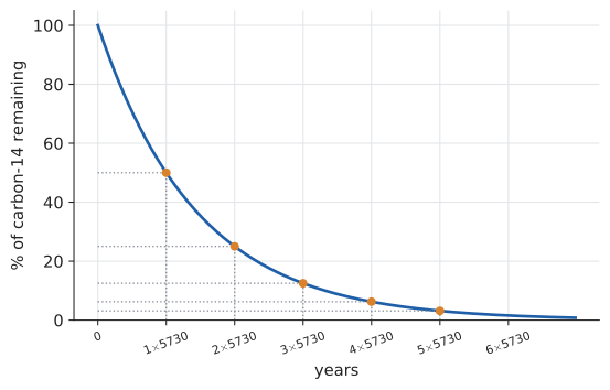
The reverse question, "how old is a sample with 30% of its carbon-14 left?", needs the exponent as the unknown. We can’t answer it with what we have yet. That is exactly what the logarithm is for, and we solve it in Section 12.5.
|
Rate versus factor, and percentage points
|
12.1.7. Where you’d use this
-
Money. Inflation of 3% a year multiplies prices by \(1.03^{20} \approx 1.81\) over 20 years: a $5 sandwich becomes about $9. The same arithmetic grows a pension pot, and works against you on unpaid debt.
-
Medicine. Caffeine has a half-life of about 5 hours in a typical adult. A 200 mg coffee at 8 a.m. leaves \(200 \times (\tfrac12)^{15/5} = 200/8 = 25\) mg in your blood at 11 p.m., about the same as a can of cola. Doctors space doses of many drugs using exactly this half-life model.
-
Computing: exponential backoff. When a network request fails, well-behaved clients wait 1 s, then 2 s, 4 s, 8 s, … before retrying, so a struggling server isn’t hammered. The tenth retry waits \(2^9 = 512\) s, over 8 minutes, which is why real implementations cap the wait.
-
Security. Every extra character multiplies the number of possible passwords. With 62 letters and digits, 8 characters give \(62^8 \approx 2.2 \times 10^{14}\) possibilities, about 6 hours of work for an attacker testing \(10^{10}\) guesses a second; 12 characters give \(62^{12} \approx 3.2 \times 10^{21}\), about 10,000 years. Length beats cleverness because length is in the exponent.
|
The king, the chessboard and the rice
An old legend has the inventor of chess ask for a reward of one grain of rice on the first square, two on the second, four on the third, and so on for all 64 squares. The total is \(2^{64} - 1 \approx 1.8 \times 10^{19}\) grains, hundreds of years of current world rice production. You will recognise \(2^{64} - 1\) as the largest unsigned 64-bit integer, |
12.2. Compound interest and the number \(e\)
12.2.1. The problem
A bank offers 100% interest a year. (Not a real bank.) Put in $1 and after a year you have $2. A rival bank says: "We pay the same rate, but we compound twice a year: 50% after six months, then 50% on the new balance." Another compounds monthly. Another daily. Another every second.
Does compounding more often make you arbitrarily rich, or is there a ceiling?
12.2.2. Intuition
Compounding more often helps, because interest starts earning interest sooner. But each split also makes the individual pieces smaller. These two effects pull against each other, and it isn’t obvious which wins.
12.2.3. The calculation
Split the year into \(n\) periods. Each period pays \(1/n\) of the annual rate, so the balance is multiplied by \(1 + 1/n\) \(n\) times:
| Compounding | \(n\) | \((1 + 1/n)^n\) |
|---|---|---|
yearly |
1 |
2 |
half-yearly |
2 |
2.25 |
quarterly |
4 |
2.441406… |
monthly |
12 |
2.613035… |
weekly |
52 |
2.692597… |
daily |
365 |
2.714567… |
hourly |
8,760 |
2.718127… |
every minute |
525,600 |
2.718279… |
The balance grows, but more and more slowly, and it levels off just above 2.718. That ceiling is the number
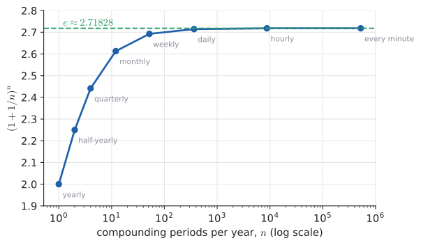
The formal definition uses a limit, which is the subject of Chapter 16:
Read "lim as \(n \to \infty\)" as "the value this expression settles towards as \(n\) grows without bound".
|
The number \(e\)
\(e \approx 2.71828\) is Euler’s number. It is irrational (its decimal expansion never repeats), like \(\pi\). Two key facts about it:
|
12.2.4. Continuous compounding in general
Suppose the annual rate is \(r\) instead of 100%, you invest a principal \(P\) for \(t\) years, and you compound \(n\) times a year. The balance is
Let \(m = n/r\). Then \(r/n = 1/m\) and \(nt = m \cdot rt\), so
That gives the continuous compounding formula
12.2.5. Worked example: three ways to compound
$1,000 at 5% a year for 10 years:
Going from annual to monthly compounding earns $18. Going from monthly to continuous earns only $1.71 more. That matches the levelling off in the table.
12.2.6. Seeing the limit numerically
import math

for n in [1, 10, 100, 10_000, 1_000_000, 10**8, 10**12, 10**16]:
    print(f"{n:>22,}  {(1 + 1/n)**n:.15f}")
print(f"{'math.e':>22}  {math.e:.15f}")
1 2.000000000000000
10 2.593742460100002
100 2.704813829421528
10,000 2.718145926824926
1,000,000 2.718280469095753
100,000,000 2.718281798347358
1,000,000,000,000 2.718523496037238
10,000,000,000,000,000 1.000000000000000
math.e 2.718281828459045
The values close in on \(e\) up to \(n = 10^8\). Then they go wrong: \(10^{12}\) is worse, and at \(10^{16}\) the answer is exactly 1. The reason is floating point. 1 + 1/n is rounded to the nearest representable double, and when \(1/n\) is below about \(1.1 \times 10^{-16}\), 1 + 1/n rounds to exactly 1.0. We return to this kind of failure in Chapter 32. The general lesson is that a numerical approach to a limit has a sweet spot. Push too far and rounding error takes over.
|
APR is not APY
Banks quote a nominal annual rate (APR) and an effective annual yield (APY). 12% APR compounded monthly gives \((1.01)^{12} - 1 = 12.68\%\) APY. If you compare loans by APR when they compound at different frequencies, you are comparing different things. |
12.2.7. Where you’d use this
Continuous compounding is how many financial models price bonds and options, but \(e\) turns up far beyond banking, wherever many small independent chances or a growth rate proportional to size are involved:
-
Biology: a bacterial population with continuous growth rate \(k = 0.7\) per hour is \(N_0 e^{0.7t}\); after 5 hours it is \(e^{3.5} \approx 33\) times larger.
-
Physics and electronics: a capacitor discharging through a resistor keeps the fraction \(e^{-t/RC}\) of its voltage. After one time constant \(t = RC\), \(e^{-1} \approx 37\%\) remains; after five, under 1%, which is why engineers treat "5 RC" as fully discharged.
-
Computing: throw \(n\) keys at random into a hash table with \(n\) buckets. Each bucket stays empty with probability \((1 - 1/n)^n \approx 1/e \approx 0.368\), so about 37% of the buckets are empty and the rest hold everything. The same limit that defined \(e\) predicts how unevenly random hashing fills a table.
|
Who found \(e\)?
Jacob Bernoulli ran into the compound-interest limit in 1683 while studying exactly this question. He showed it was between 2 and 3. Leonhard Euler later gave it the letter \(e\) (probably not after himself, despite the popular story), computed it to more than 20 decimal places and proved it irrational. The same number turns up in probability: if you shuffle \(n\) letters into \(n\) envelopes at random, the chance that none lands in the right envelope approaches \(1/e \approx 0.368\). |
12.3. The logarithm: "what power?"
12.3.1. The problem
From Section 12.1 you can answer "\(2^{10}\) is what?" (1,024). Now turn the question round:
\(2^{?} = 1024\). What power of 2 gives 1,024?
That is the question a logarithm answers. The answer is 10, and we write
Questions like this come up constantly. How many years until my investment doubles? How old is this fossil? How many times can I halve a list of a million items before one item is left? How many bits does it take to count to a billion? Each asks for an unknown exponent.
12.3.2. Definition
|
Logarithm
For a base \(b > 0\), \(b \ne 1\), and a positive number \(x\):
\[\log_b x = y \quad\Longleftrightarrow\quad b^{y} = x.\]
Read \(\log_b x\) as "log base \(b\) of \(x\)". It is the exponent you put on \(b\) to get \(x\). In the equation \(b^y = x\):
The double arrow \(\Longleftrightarrow\) means "if and only if": each statement implies the other, so they are two ways of saying the same thing. |
The word to hold onto: a logarithm is an exponent. Every fact about logarithms is a fact about exponents written the other way round.
12.3.3. Worked examples: evaluating logs by hand
Each of these is answered by asking "what power?":
One more, a bit harder: \(\log_8 32\). Both 8 and 32 are powers of 2: \(8 = 2^3\) and \(32 = 2^5\). We want \(y\) with
So \(\log_8 32 = 5/3\). Check: \(8^{5/3} = (\sqrt[3]{8})^5 = 2^5 = 32\). Correct.
12.3.4. The log function and its graph
Because \(y = b^x\) is one-to-one, it has an inverse function (Chapter 11), and that inverse is \(y = \log_b x\). Inverse functions undo each other:
The graph of an inverse function is the original graph reflected in the line \(y = x\). Every point \((p, q)\) on \(y = 2^x\) becomes the point \((q, p)\) on \(y = \log_2 x\).
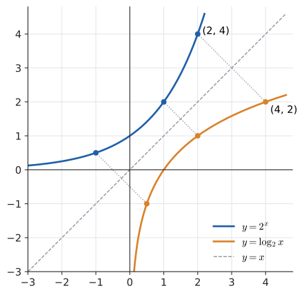
Swapping the roles of \(x\) and \(y\) in the exponential’s properties gives the logarithm’s properties:
| \(y = b^x\) (\(b > 1\)) | \(y = \log_b x\) (\(b > 1\)) | |
|---|---|---|
Domain |
all reals |
\(x > 0\) only |
Range |
\(y > 0\) |
all reals |
Key point |
\((0, 1)\) |
\((1, 0)\) |
Asymptote |
horizontal, \(y = 0\) |
vertical, \(x = 0\) |
Growth |
faster and faster |
slower and slower, but never stops |
The last row matters a lot in computing. \(\log_2 x\) does keep increasing without limit, but extremely slowly. \(\log_2\) of a thousand is about 10, of a million about 20, of a billion about 30. Multiplying the input by 1,000 adds only about 10 to the output. That is why an algorithm that takes \(\log n\) steps scales so well.
|
Logs of zero and negative numbers do not exist (in the reals)
\(\log_b x\) is defined only for \(x > 0\), because a positive base raised to any real power is positive. \(\log_{10}(-100)\) has no real answer, and \(\log 0\) is undefined. (As \(x \to 0^+\) the log heads to \(-\infty\).) In code, |
12.4. The laws of logarithms, derived
12.4.1. The problem
Before calculators, multiplying two seven-digit numbers by hand was slow and easy to get wrong, while adding them was fast. Navigators, astronomers and engineers wanted a way to turn multiplication into addition. Logarithms did that, and the reason is a single exponent law.
12.4.2. Why it works: the derivations
The log laws aren’t new rules to memorise. Each is an exponent law from Chapter 3 read backwards. In everything below, \(b > 0\), \(b \ne 1\), and \(M, N > 0\).
Product law. Let \(m = \log_b M\) and \(n = \log_b N\). By definition, \(b^m = M\) and \(b^n = N\). Then
Quotient law. Same setup:
Power law. For any real \(k\):
Change of base. Suppose you need \(\log_2 50\) but your calculator only has \(\log_{10}\) and \(\ln\). Let \(y = \log_b x\), so \(b^y = x\). Take log base \(c\) (any convenient base) of both sides:
So
In words: every logarithm is a constant multiple of every other. \(\log_2 x = \log_{10} x / \log_{10} 2 \approx 3.3219 \log_{10} x\). Changing the base just rescales the vertical axis of the graph.
|
The laws of logarithms
For \(b, c > 0\), \(b, c \ne 1\), \(M, N > 0\), and any real \(k\):
|
12.4.3. Common, natural and binary logarithms
Three bases account for nearly every logarithm you will meet.
|
Common, natural and binary logarithms
In code: Python’s |
Some values worth recognising:
\(\log_{10} 2 \approx 0.301\) says \(2^{10} = 1024 \approx 10^3\): ten doublings add about three decimal digits. That is the familiar kilo/kibi relationship. Big-O notation doesn’t care about the base of a log, because by change of base \(\log_2 n\) and \(\log_{10} n\) differ only by a constant factor.
12.4.4. Where you’d use this
-
Counting digits. The number of decimal digits of a positive integer \(N\) is \(\lfloor \log_{10} N \rfloor + 1\). How many digits does \(2^{100}\) have? \(\log_{10} 2^{100} = 100 \log_{10} 2 \approx 30.10\), so 31 digits, without computing the number.
-
Music. Pitch is logarithmic: each octave doubles the frequency, and each of the 12 semitones in an octave multiplies it by \(2^{1/12} \approx 1.0595\). The interval from 440 Hz (concert A) to 660 Hz is \(12 \log_2(660/440) = 12 \log_2 1.5 \approx 7.02\) semitones: a perfect fifth.
-
Photography. Each "stop" of exposure doubles or halves the light, so camera settings are a base-2 log scale. Going from f/4 to f/8 doubles the aperture’s f-number, which quarters the aperture’s area: two stops darker.
-
Computing. \(\log_2\) counts bits and halvings (see Section 12.9); the product law is why adding log-probabilities replaces multiplying tiny probabilities in spam filters and language models.
12.4.5. The method: expanding and condensing
Input: an expression involving logs of products, quotients and powers (to expand), or a sum and difference of logs with coefficients (to condense).
Steps (expanding):
-
Rewrite roots as fractional powers: \(\sqrt[n]{u} = u^{1/n}\).
-
Split products into sums and quotients into differences (product and quotient laws).
-
Bring exponents down as coefficients (power law).
-
Evaluate any logs of known powers of the base (\(\log_b b^k = k\)).
Steps (condensing): run the steps backwards. First move coefficients up as exponents, then combine sums into products and differences into quotients, and finish with a single log.
Output: an equivalent expression. Check by plugging in a number on both sides.
12.4.6. Worked examples
Expand \(\log_2\!\left(\dfrac{8x^3}{\sqrt{y}}\right)\):
Condense \(2\ln a + \ln b - 3\ln c\) to a single log:
Change of base: compute \(\log_3 20\) with a calculator that only has \(\ln\):
Check: \(3^{2.726833}\) should be 20. \(3^{2} = 9\) and \(3^{3} = 27\), so an exponent between 2 and 3 that lands closer to 3 is about right.
|
Laws that do not exist
The commonest log mistakes are made-up "laws" that look plausible:
Quick test: plug in numbers. \(\log_{10}(10 + 10) = \log_{10} 20 \approx 1.301\), but \(\log_{10}10 + \log_{10}10 = 2\). |
|
Slide rules and log tables
John Napier published logarithms in 1614, and Henry Briggs soon produced base-10 tables. For three and a half centuries, scientists multiplied by looking up two logs, adding them, and looking up the antilog. A slide rule builds the same idea into hardware. Its scales are marked at distances proportional to \(\log x\), so sliding one scale along another adds lengths, which multiplies numbers. The engineers on the Apollo programme carried slide rules. Laplace said logarithms, "by shortening the labours, doubled the life of the astronomer." |
12.5. Solving exponential and logarithmic equations
12.5.1. The problem
Now we can answer the questions we set aside earlier. When will $1,000 at 6% become $2,000? How old is a bone with 30% of its carbon-14 left? In each the unknown is in the exponent, and the way to get it down is to take a logarithm of both sides.
12.5.2. Why it works
Taking logs is allowed because \(\log\) is a function: equal inputs give equal outputs, so if \(A = B\) (both positive) then \(\log A = \log B\). Then the power law moves the unknown exponent down to the main line, where ordinary algebra (Chapter 5) can reach it:
The arrow \(\Longrightarrow\) means "implies".
12.5.3. The method
Input: an equation with the unknown in one or more exponents.
Steps:
-
Isolate the exponential term \(b^{(\ldots)}\) on one side, using ordinary algebra (subtract constants, divide by coefficients).
-
Same-base shortcut: if both sides can be written as powers of the same base, set the exponents equal and skip to step 5.
-
Take logs of both sides. \(\ln\) is the usual choice, or \(\log_b\) when the base is \(b\), since that cancels in one step.
-
Bring down the exponent with the power law.
-
Solve the resulting linear (or occasionally quadratic) equation for the unknown.
-
Check by substituting back. Also confirm the answer is sensible: a time that comes out negative, say, means something went wrong.
Output: exact solution(s) in terms of logs, and a decimal approximation.
12.5.4. Worked example 1: a pure exponential
Solve \(2^{x} = 50\).
Check: \(2^5 = 32\) and \(2^6 = 64\), so the answer has to be between 5 and 6. \(x \approx 5.64\) passes. (Equivalently, \(x = \log_2 50\).)
12.5.5. Worked example 2: isolate first
Solve \(3 \cdot 5^{2x - 1} = 400\).
|
Isolate before taking logs
A frequent wrong move is to take logs straight away and write \(\ln(3 \cdot 5^{2x-1}) = (2x-1)\ln 15\). The 3 is not part of the base. Either isolate first (as above) or use the product law properly: \(\ln 3 + (2x-1)\ln 5 = \ln 400\). Both routes give the same answer. And if the equation is \(5^{x} + 3 = 20\), subtract the 3 before logging, because \(\ln(5^x + 3)\) can’t be simplified. |
12.5.6. Worked example 3: carbon dating
A bone has 30% of the carbon-14 that living tissue has. How old is it? (Half-life 5,730 years.)
The two negative logs cancel to give a positive age. Sanity check: 30% is between 50% (one half-life) and 25% (two half-lives), and 9,953 years is between 5,730 and 11,460.
12.5.7. Worked example 4: doubling time and the rule of 72
How long does money take to double at 6% compounded annually?
Bankers use the rule of 72: doubling time \(\approx 72 / (\text{rate in percent})\), here \(72/6 = 12\). Why does it work? For small \(r\), \(\ln(1 + r) \approx r\) (you’ll see why in Chapter 17), so
69.3 would be the more accurate constant for small rates. 72 is used because it divides evenly by 2, 3, 4, 6, 8, 9 and 12, and because it partly corrects for \(\ln(1+r)\) being a little less than \(r\) at typical rates of 6–10%.
12.5.8. Worked example 5: a logarithmic equation
Solve \(\log_2 x + \log_2(x - 2) = 3\).
(Factoring quadratics is covered in Chapter 8.)
Check: \(x = 4\) gives \(\log_2 4 + \log_2 2 = 2 + 1 = 3\). Correct. \(x = -2\) gives \(\log_2(-2)\), which is undefined, so we reject it. It is an extraneous solution: condensing the logs widened the domain, because \(x(x - 2) > 0\) also allows \(x < 0\).
|
Extraneous solution
An extraneous solution is a value produced by a valid-looking algebraic process that does not actually satisfy the original equation. Steps such as squaring both sides or combining logarithms can introduce them, because they can enlarge the set of allowed inputs. Always substitute back into the original equation. |
12.5.9. Alternative approaches and choosing a method
-
Same-base matching. \(4^{x} = 8\) becomes \(2^{2x} = 2^{3}\), so \(x = 3/2\). You get an exact answer and need no calculator. Use it whenever both sides are obviously powers of one base.
-
Logarithms. This is the general method for a single exponential term, or one exponential on each side (\(3^{x} = 7^{x-1}\) becomes \(x\ln 3 = (x - 1)\ln 7\), which is linear in \(x\)).
-
Substitution. \(4^x - 3 \cdot 2^x - 4 = 0\) is a quadratic in disguise. Let \(u = 2^x\), so \(4^x = u^2\), giving \(u^2 - 3u - 4 = 0\), \((u-4)(u+1) = 0\). \(u = 2^x\) must be positive, so \(u = 4\) and \(x = 2\).
-
Numerical or graphical methods. Equations that mix an exponential with a polynomial, such as \(2^x = x^{10}\) or \(e^{x} = 3x\), cannot be solved with logs and algebra alone. Plot both sides, or use bisection or Newton’s method (Chapter 32). Log-transforming can still help: \(2^x = x^{10}\) is equivalent to \(x\ln 2 = 10 \ln x\), a nicer function to bisect.
The decision rule: same base → match exponents; one exponential term → isolate and log; exponentials of related bases → substitute; exponential mixed with polynomial → numerical.
12.5.10. Implementation
import math

def solve_exponential(a, b, c):
    """Solve a * b**x = c for x. Requires a, c of the same sign, b > 0, b != 1."""
    if b <= 0 or b == 1:
        raise ValueError("base must be positive and not 1")
    ratio = c / a                     # step 1: isolate b**x
    if ratio <= 0:
        raise ValueError("no real solution: b**x is always positive")
    return math.log(ratio) / math.log(b)   # steps 3-5

x = solve_exponential(3, 5, 400)      # 3 * 5**x = 400
print(round(x, 6), 3 * 5**x)
print(round(solve_exponential(1, 1.06, 2), 4))   # doubling time at 6%
3.0401 400.0000000000001 11.8957
(The first line solves for the whole exponent \(2x - 1 = 3.0401\). The final digit in 400.0000000000001 is floating-point rounding.)
12.5.11. Where you’d use this
Every "how long until …?" question about an exponential process is solved this way:
-
Debt. An unpaid credit-card balance at 2% a month (about 24% APR) doubles when \(1.02^t = 2\), i.e. after \(t = \ln 2 / \ln 1.02 \approx 35\) months: under three years.
-
Medicine. With caffeine’s 5-hour half-life, when does a 200 mg dose fall below 50 mg? \(200 (\tfrac12)^{t/5} = 50\) gives \((\tfrac12)^{t/5} = \tfrac14\), so \(t/5 = 2\) and \(t = 10\) hours. Pharmacologists use the same equation to decide when a drug has effectively cleared (about 5 half-lives, when under 4% remains).
-
Technology forecasts. If computing power doubles every 2 years, how long until it is 1,000 times greater? \(2^{t/2} = 1000\) gives \(t = 2\log_2 1000 \approx 19.9\) years: roughly 20 years for three orders of magnitude.
12.6. Logarithmic scales
12.6.1. The problem
The quietest sound a human can hear and the sound of a jet engine at 30 m differ in intensity by a factor of about \(10^{14}\). Earthquakes span a similar range of energies. Hydrogen-ion concentrations in everyday liquids run from about 1 down to \(10^{-14}\) moles per litre. Put any of these on an ordinary linear axis and everything except the biggest values gets squashed into an invisible sliver near zero.
12.6.2. Intuition
A logarithmic scale places each value at a position proportional to its logarithm. Equal distances then represent equal ratios, not equal differences. On a base-10 log scale, 1 → 10 → 100 → 1,000 are evenly spaced, each one "decade" apart. Our senses work roughly like this: a sound ten times as intense doesn’t seem ten times as loud.
12.6.3. Three famous scales
Decibels (sound, signals). The sound intensity level is Try it: Decibels and power ratios.
where \(I_0 = 10^{-12}\ \text{W/m}^2\) is the threshold of hearing. Multiplying intensity by 10 adds 10 dB, and doubling it adds \(10\log_{10}2 \approx 3.01\) dB. Engineers use dB for any power ratio: amplifier gain, Wi-Fi signal strength (dBm), the signal-to-noise ratio of an ADC.
Worked example. A sound is 85 dB. How many times more intense than a 60 dB sound is it? Try it: 25 dB as a ratio.
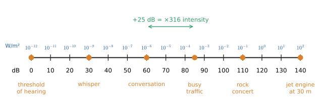
Earthquake magnitude. The Richter scale, and the moment-magnitude scale that replaced it, is logarithmic. Each whole number up means about 10 times the ground-motion amplitude and about \(10^{1.5} \approx 31.6\) times the energy released. A magnitude 7 quake releases about \(31.6^2 \approx 1000\) times the energy of a magnitude 5.
pH (chemistry).
where \(\lbrack\mathrm{H}^{+}\rbrack\) is the hydrogen-ion concentration in moles per litre. The minus sign makes everyday values positive. Pure water has a hydrogen-ion concentration of \(10^{-7}\), so pH 7. Lemon juice at pH 2 has \(10^{5} = 100{,}000\) times the hydrogen-ion concentration of water.
|
Logarithmic scale
A logarithmic scale positions a value \(v\) at distance proportional to \(\log v\). Equal steps along it are equal multiplications. A decade is a factor of 10, and an octave (in music, and in frequency analysis) is a factor of 2. |
12.6.4. Log plots: semi-log and log-log
Graphs can use a log scale on one axis or both.
-
Semi-log plot (log scale on the \(y\)-axis only). An exponential \(y = a b^x\) becomes a straight line: \(\log y = \log a + x\log b\), which is linear in \(x\) with slope \(\log b\). Use it to check whether data is exponential and to read off growth rates. Epidemic curves and Moore’s-law charts are drawn this way.
-
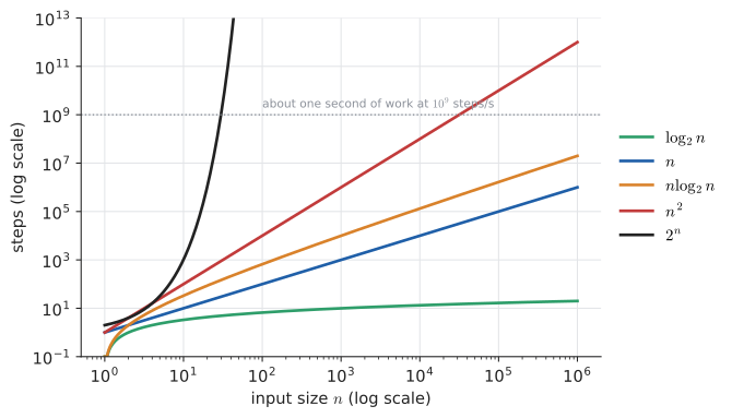
Log-log plot (both axes logarithmic). A power law \(y = a x^k\) becomes a straight line: \(\log y = \log a + k\log x\), with slope \(k\). Use it to find exponents in power laws, for example when checking the empirical complexity of an algorithm.
|
A log-log plot is a practical tool for performance work. Time your function at \(n = 1000, 2000, 4000, \ldots\), plot time against \(n\) on log-log axes, and measure the slope. A slope near 1 means linear, near 2 means quadratic. A slope that keeps increasing means something worse than polynomial is going on. |
|
Reading log axes
|
|
Benford’s law
In many real-world datasets (populations, river lengths, invoice amounts) the leading digit is 1 about 30.1% of the time and 9 only about 4.6% of the time. The probability of leading digit \(d\) is \(\log_{10}(1 + 1/d)\): \(\log_{10}2 \approx 0.301\) for \(d = 1\). This happens when data is spread evenly on a log scale. Forensic accountants use departures from Benford’s law to flag fabricated figures. |
12.7. Exponential models and fitting them to data
12.7.1. The problem
You have data, say case counts of a spreading infection, users of a new app, or the runtime of a brute-force solver as the input grows. It curves upward. Is it exponential? If so, what are \(a\) and \(b\), what is the doubling time, and what does the model predict?
12.7.2. Intuition: straighten the curve
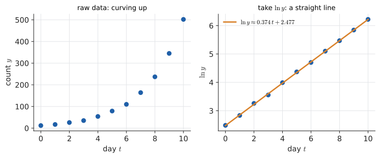
You know how to fit a straight line (Chapter 5). Logarithms turn an exponential into a straight line, so take the log of the data, fit a line, and convert back.
If \(y = a e^{kt}\), then
This is a line in the variables \(t\) and \(\ln y\), with slope \(k\) and intercept \(\ln a\). The base-\(e\) form \(a e^{kt}\) is the one scientists prefer. It is the same family as \(a b^t\), with \(b = e^{k}\) (so \(k = \ln b\)). \(k\) is called the continuous growth rate.
12.7.3. Worked example: fitting by hand from two points
A culture has 500 cells at hour 2 and 4,000 cells at hour 5. Find \(y = a e^{kt}\). Try it: Fit y = a·e^(kt).
So \(y = 125\, e^{0.6931\,t} = 125 \cdot 2^{t}\). The culture doubles every hour, and there were 125 cells at \(t = 0\).
12.7.4. Worked example: fitting many points
With real, noisy data, use all the points. Fit a least-squares line to \((t, \ln y)\). (Least squares is covered properly in Chapter 31. For now, think of it as "the line that best goes through the cloud of points".) Try it: Fit the case counts.
import numpy as np

days  = np.arange(0, 11)
cases = np.array([12, 17, 26, 35, 54, 79, 110, 164, 237, 345, 502])

k, ln_a = np.polyfit(days, np.log(cases), 1)   # fit ln y = k t + ln a
a = np.exp(ln_a)
print(f"k = {k:.4f} per day, a = {a:.2f}")
print(f"daily growth factor = {np.exp(k):.4f}")
print(f"doubling time = {np.log(2) / k:.2f} days")
print(f"model at day 14: {a * np.exp(k * 14):.0f}")
Try it: Run this in your browser.
k = 0.3740 per day, a = 11.91
daily growth factor = 1.4535
doubling time = 1.85 days
model at day 14: 2238
12.7.5. Choosing a model
How can you tell whether to use a linear, exponential or power-law model? Transform the data and see which version comes out straight:
| Plot | Straight line means | Model |
|---|---|---|
\(y\) vs \(x\) |
constant differences |
linear \(y = mx + c\) |
\(\ln y\) vs \(x\) (semi-log) |
constant ratios |
exponential \(y = a e^{kx}\) |
\(\ln y\) vs \(\ln x\) (log-log) |
constant elasticity |
power law \(y = a x^{p}\) |
12.7.6. Failure modes
|
Exponential growth always ends
Nothing physical grows exponentially for ever. Infections run out of susceptible people, bacteria run out of food, and apps run out of potential users. Real growth usually follows an S-shaped logistic curve. It looks exponential early on, then bends over and levels off at a carrying capacity. Extrapolating an exponential fit far beyond the data is one of the commonest forecasting errors there is. The rumour from the start of this chapter can’t reach more than 8 billion people. A technical caveat: fitting a line to \(\ln y\) gives every point equal weight on the log scale. That is reasonable when the noise is proportional to the value, but it is not the same as least squares on \(y\) itself. |
|
Exponential decay all around you
Newton’s law of cooling (a hot coffee’s excess temperature over the room decays exponentially), drug elimination from the bloodstream, a capacitor discharging through a resistor, light dimming as it passes through water, and the "exponential moving average" behind smoothed metrics on a dashboard all follow \(y = a e^{-kt}\). They share a mechanism: the rate of change is proportional to the current amount. In Chapter 17 that becomes the differential equation \(y' = ky\), and \(e^{kt}\) is its solution. |
|
Two-point exponential fit
Drag points on a scatter plot and switch the \(y\)-axis between linear and log scale. Watch exponential data straighten under the log. Fit a line on the log view and see the fitted \(a\) and \(k\) (and doubling time) update live. Then add a logistic "saturation" and watch the fit’s predictions go badly wrong beyond the data. Try it: Exponential fit to data |
12.8. Why exponentials beat polynomials
12.8.1. The problem
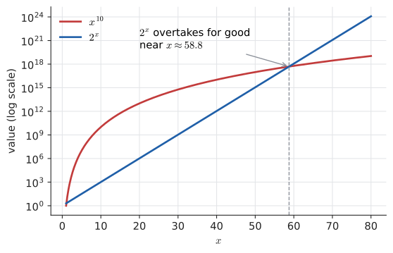
\(x^{10}\) is a huge polynomial. At \(x = 10\) it is ten billion, while \(2^{10}\) is only 1,024. Is \(x^{10}\) bigger for good? An algorithm that takes \(n^{10}\) steps would be useless in practice, but theory still calls it "efficient" (polynomial), while \(2^n\) is "intractable". Why does exponential rank as worse?
12.8.2. Intuition: ratios
Compare how each function changes when \(x\) goes up by 1:
The exponential multiplies itself by 2 at every step for ever. The polynomial’s step-to-step growth factor shrinks towards 1. Eventually it is below 2 and stays there. Once the polynomial is growing by less than 2× per step and the exponential by exactly 2×, the exponential closes any gap and pulls ahead.
12.8.3. Making it precise with logs
Take logs of both to compare them:
The left side is a straight line. The right side is a log curve, which grows more slowly than any line. A line with any positive slope eventually overtakes \(10\ln x\) and never falls back. For \(2^x\) vs \(x^{10}\), solving \(x \ln 2 = 10 \ln x\) numerically gives crossover points at \(x \approx 1.078\) and \(x \approx 58.77\). Beyond about 58.8, \(2^x\) wins for ever.
The general statements, which Chapter 16 makes rigorous:
-
For any base \(b > 1\) and any power \(p\), however large: \(b^{x}\) eventually exceeds \(x^{p}\).
-
For any power \(p > 0\), however small: \(x^{p}\) eventually exceeds \(\log x\). Even \(x^{0.01}\) beats \(\ln x\) in the end, though only for astronomically large \(x\).
That gives the growth hierarchy:
where \(\ll\) means "is eventually negligible compared with".
12.9. Logarithms in computer science
This section collects the places where logarithms do real work in computing. The single most useful idea is this:
\(\log_2 n\) is the number of times you can halve \(n\) before reaching 1.
12.9.1. Binary search: counting halvings
Searching a sorted array of \(n\) items, each comparison throws away half of what remains. After \(k\) comparisons, about \(n / 2^{k}\) items are left. We stop when one item is left: Try it: Binary search on a billion.
So binary search needs about \(\lceil \log_2 n \rceil\) comparisons. \(\lceil \cdot \rceil\) is the ceiling, which rounds up to the next integer. For a billion items that is
comparisons, where linear search needs up to a billion.
Input: a positive number \(n\).
Steps:
-
Write \(n\) in powers of 1,000: \(n \approx m \times 1000^{j}\).
-
Each factor of 1,000 contributes about 10 (because \(2^{10} = 1024 \approx 1000\)), so add \(10j\).
-
Add \(\log_2 m\) for the leftover \(m\) (\(\log_2 2 = 1\), \(\log_2 4 = 2\), \(\log_2 8 = 3\), …, \(\log_2 500 \approx 9\)).
Output: \(\log_2 n \approx 10j + \log_2 m\). Example: 64 million \(= 64 \times 1000^{2}\), so \(\approx 20 + 6 = 26\). (The exact value is 25.93.)
Try it: Estimate log₂ in your head.
12.9.2. Tree height
A complete binary tree of height \(h\) (\(h\) levels of edges below the root) holds up to Try it: Tree height and B-trees.
nodes. (That sum is a geometric series, Chapter 14.) So a balanced tree holding \(n\) keys needs height only about \(\log_2 n\). That is why a balanced binary search tree, a heap or a red–black tree gives \(O(\log n)\) lookups and inserts. A B-tree with branching factor \(B\) has height about \(\log_B n\). With \(B = 500\), a billion keys fit in a tree of height \(\log_{500} 10^9 = 9/\log_{10}500 \approx 3.3\), so in practice four levels, four disk reads. Try it: Merge sort’s log₂ n levels.
Merge sort splits the list in half repeatedly, giving \(\log_2 n\) levels of splitting with \(n\) work per level, for a total of \(O(n \log n)\) (Chapter 24 counts this more carefully).
12.9.3. Bits needed to represent \(n\)
With \(k\) bits you can write \(2^{k}\) different values, 0 to \(2^{k} - 1\). To store the integers 0 to \(n\) you need the smallest \(k\) with \(2^{k} > n\):
where \(\lfloor \cdot \rfloor\) is the floor, which rounds down. For example, 1,000,000 needs \(\lfloor 19.93 \rfloor + 1 = 20\) bits. Likewise the number of decimal digits in \(n\) is \(\lfloor \log_{10} n \rfloor + 1\).
import math

for n in [1, 255, 256, 1_000_000, 10**9]:
    print(n, math.floor(math.log2(n)) + 1, n.bit_length())
1 1 1 255 8 8 256 9 9 1000000 20 20 1000000000 30 30
|
Floating-point logs at exact powers
|
12.9.4. Comparing growth rates
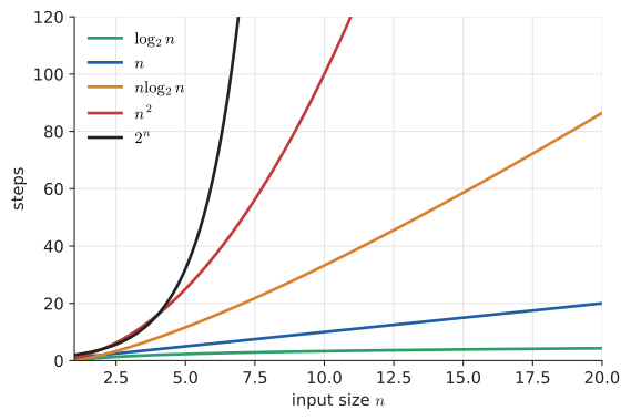
Here is how many basic steps algorithms of different complexity need, and how long they’d take at \(10^{9}\) steps per second:
| \(n\) | \(\log_2 n\) | \(n\) | \(n \log_2 n\) | \(n^{2}\) | \(2^{n}\) |
|---|---|---|---|---|---|
10 |
3.3 |
10 |
33 |
100 |
1,024 |
100 |
6.6 |
100 |
664 |
10,000 |
\(1.3 \times 10^{30}\) |
1,000 |
10.0 |
1,000 |
9,966 |
\(10^{6}\) |
\(1.1 \times 10^{301}\) |
\(10^{6}\) |
19.9 |
\(10^{6}\) |
\(2.0 \times 10^{7}\) |
\(10^{12}\) (17 min) |
— |
\(10^{9}\) |
29.9 |
\(10^{9}\) (1 s) |
\(3.0 \times 10^{10}\) (30 s) |
\(10^{18}\) (32 years) |
— |
\(2^{100}\) steps at a billion per second would take about \(4 \times 10^{13}\) years, thousands of times the age of the universe. That is why "exponential time" means "infeasible" for anything but small inputs.
12.9.5. Information: how many bits is a choice worth?
How many yes/no questions does it take to identify one of 8 equally likely possibilities? Each well-chosen question halves the candidates: 8 → 4 → 2 → 1. That is 3 questions, and \(3 = \log_2 8\). In general, picking one of \(N\) equally likely options conveys
A fair coin flip is 1 bit. A roll of a fair die is \(\log_2 6 \approx 2.585\) bits. A random 12-character password from 94 printable characters has \(12 \log_2 94 \approx 78.7\) bits of entropy. The game Twenty Questions can distinguish \(2^{20} \approx 1{,}048{,}576\) objects.
Claude Shannon generalised this to unequal probabilities. An outcome of probability \(p\) carries \(-\log_2 p\) bits of surprise, and the average surprise of a source is its entropy. That is the foundation of compression (Huffman coding, arithmetic coding) and of the cross-entropy loss used to train classifiers (Chapter 29).
12.9.6. Products to sums: log probabilities
Multiply a thousand probabilities of 0.01 each, as a language model or a naive Bayes classifier might when scoring a long document:
The smallest positive double is about \(5 \times 10^{-324}\), so the product underflows to 0.0, and every candidate document scores the same zero. The fix is to work in logs: the product law turns the product into a sum,
which is a perfectly ordinary floating-point number. (\(\prod\) is the product symbol, the multiplicative cousin of \(\sum\). Read \(\prod_i p_i\) as "multiply all the \(p_i\) together". \(\sum_i \ln p_i\) means "add up all the \(\ln p_i\)".) Since \(\ln\) is increasing, comparing log-probabilities gives the same ranking as comparing probabilities. Log-likelihood, log-loss and log-odds all exist for this reason.
import math

probs = [0.01] * 1000
product = 1.0
for p in probs:
    product *= p
print(product)                          # underflow
print(sum(math.log(p) for p in probs))  # fine
0.0 -4605.17018598815
12.9.7. A teaser: log-sum-exp and softmax
A classifier produces scores \(z_1, \ldots, z_K\) ("logits") and turns them into probabilities with the softmax function:
If any \(z_i\) is around 1,000, then \(e^{1000}\) overflows to infinity and the result is nan. The standard fix uses an exponent law. For any constant \(m\),
Choose \(m = \max_j z_j\). Every exponent \(z_j - m\) is then at most 0, so nothing overflows and at least one term equals 1. The same trick computes \(\log\sum_j e^{z_j} = m + \log\sum_j e^{z_j - m}\) safely. This is the log-sum-exp function, which appears throughout machine learning.
import numpy as np

def softmax_naive(z):
    e = np.exp(z)
    return e / e.sum()

def softmax_stable(z):
    e = np.exp(z - np.max(z))   # shift so the largest exponent is 0
    return e / e.sum()

z = np.array([1000.0, 1001.0, 1002.0])
with np.errstate(over="ignore", invalid="ignore"):
    print(softmax_naive(z))
print(softmax_stable(z))
[nan nan nan] [0.09003057 0.24472847 0.66524096]
|
Halving explorer
Pick \(n\) with a slider (1 to \(10^{12}\)) and watch binary search on a bar of \(n\) items. The bar halves on each step and a counter shows comparisons. Beside it, show \(\log_2 n\), the bits needed for \(n\), and the height of a balanced tree holding \(n\) keys, so the reader sees all three are the same number. Try it: Halving explorer |
|
Growth-race plotter
Plot \(\log n\), \(n\), \(n\log n\), \(n^k\) (with \(k\) on a slider) and \(b^n\) (with \(b\) on a slider). Toggle linear, semi-log and log-log axes. Find where \(1.01^n\) finally overtakes \(n^{3}\). (It happens near \(n \approx 2{,}340\).) |
12.10. Interactive tools
Browser tools on the companion website that go with this chapter. Each example link in the chapter opens one of them with that example already set up.
12.11. Exercises
Recognition
-
Which of these are exponential functions? (a) \(y = 3x^2\) (b) \(y = 3 \cdot 2^x\) (c) \(y = (0.7)^x\) (d) \(y = x^x\) (e) \(y = 5\).
-
The table \(x = 0, 1, 2, 3\) has \(y = 6, 9, 13.5, 20.25\). Linear or exponential? Find the formula.
-
Write in exponential form: (a) \(\log_3 81 = 4\) (b) \(\ln x = 2\). Write in log form: (c) \(10^{-2} = 0.01\) (d) \(e^{0} = 1\).
-
Evaluate without a calculator: (a) \(\log_2 64\) (b) \(\log_{10} 0.0001\) (c) \(\log_9 3\) (d) \(\ln e^{7}\) (e) \(\log_{27} 9\).
Application
-
Expand \(\log_{10}\!\left(\dfrac{100\, x^2}{\sqrt[3]{y}}\right)\).
-
Condense to one log: \(\tfrac12\ln x - 2\ln(x+1) + \ln 3\).
-
Solve: (a) \(5^{x} = 200\) (b) \(2 \cdot 3^{x+1} = 54\) (c) \(e^{2x} = 7\) (d) \(4^{x} = 32\).
-
$5,000 is invested at 4% a year. Find the balance after 15 years if compounded (a) annually (b) continuously. How long does it take to double in case (a)?
-
A drug has a half-life of 6 hours. What fraction remains after 24 hours? After how many hours is only 10% left?
-
Solve \(\log_3(x + 6) + \log_3 x = 3\), and check for extraneous solutions.
Problem solving
-
A sound meter reads 72 dB in a café and 96 dB at a concert. How many times more intense is the concert?
-
A sorted table has 50 million rows. At most how many comparisons does binary search need? How many bits are needed to store a row index?
-
Two measurements of a population: 2,000 in 2010, 2,900 in 2020. Fit \(P = a e^{k(t - 2010)}\). Predict 2030 and give the doubling time.
-
Show that \(\log_b x \cdot \log_x b = 1\) for valid \(b, x\).
-
A website’s traffic doubles every 4 months. Write the monthly growth factor exactly, and give the percentage monthly growth rate.
-
An algorithm takes \(n^{3}\) steps and another takes \(1.5^{n}\) steps. Use logs and a quick search (by hand or in code) to estimate the largest \(n\) for which the exponential one is still faster, beyond the trivial region near \(n = 1\).
Answers
-
(b) and (c) are exponential. (a) is a power function. (d) has the variable in the base and the exponent, so it isn’t of the form \(ab^x\). (e) is constant (\(b = 1\) is excluded).
-
Ratios: \(9/6 = 13.5/9 = 20.25/13.5 = 1.5\). Constant ratio, so exponential: \(y = 6(1.5)^{x}\).
-
(a) \(3^{4} = 81\) (b) \(e^{2} = x\) (c) \(\log_{10} 0.01 = -2\) (d) \(\ln 1 = 0\).
-
(a) 6 (\(2^6 = 64\)) (b) \(-4\) (c) \(\tfrac12\) (\(9^{1/2} = 3\)) (d) 7 (e) \(27^{y} = 9 \Rightarrow 3^{3y} = 3^{2} \Rightarrow y = \tfrac23\).
-
\(\log 100 + \log x^2 - \log y^{1/3} = 2 + 2\log x - \tfrac13\log y\).
-
\(\ln\sqrt{x} - \ln(x+1)^2 + \ln 3 = \ln\!\left(\dfrac{3\sqrt{x}}{(x+1)^2}\right)\).
-
(a) \(x = \ln 200 / \ln 5 = 5.298317/1.609438 \approx 3.292\). (b) \(3^{x+1} = 27 = 3^3 \Rightarrow x + 1 = 3 \Rightarrow x = 2\). (c) \(2x = \ln 7 \Rightarrow x = 1.945910/2 \approx 0.973\). (d) \(2^{2x} = 2^{5} \Rightarrow x = 5/2\).
-
(a) \(5000(1.04)^{15} = 5000 \times 1.800944 \approx \$9{,}004.72\). (b) \(5000e^{0.6} = 5000 \times 1.822119 \approx \$9{,}110.59\). Doubling: \(t = \ln 2/\ln 1.04 = 0.693147/0.039221 \approx 17.67\) years (rule of 72: 18).
-
24 hours is 4 half-lives, so \((1/2)^4 = 1/16 = 6.25\%\) remains. For 10%: \((1/2)^{t/6} = 0.1 \Rightarrow t = 6\ln 0.1/\ln 0.5 = 6 \times 3.321928 \approx 19.93\) hours.
-
\(\log_3\big(x(x+6)\big) = 3 \Rightarrow x^2 + 6x = 27 \Rightarrow x^2 + 6x - 27 = 0 \Rightarrow (x + 9)(x - 3) = 0\). \(x = 3\) checks: \(\log_3 9 + \log_3 3 = 2 + 1 = 3\). \(x = -9\) is extraneous (log of a negative).
-
\(96 - 72 = 24 = 10\log_{10}(I_1/I_2)\), so \(I_1/I_2 = 10^{2.4} \approx 251\).
-
\(\log_2(5 \times 10^{7}) \approx 25.58\), so 26 comparisons. Indices 0 to 49,999,999 need \(\lfloor\log_2 49{,}999{,}999\rfloor + 1 = 25 + 1 = 26\) bits.
-
\(a = 2000\). \(e^{10k} = 1.45 \Rightarrow k = \ln 1.45/10 = 0.371564/10 \approx 0.037156\). 2030: \(2000e^{20k} = 2000 \times 1.45^{2} = 4{,}205\). Doubling time \(\ln 2/k \approx 18.65\) years.
-
By change of base, \(\log_b x = \dfrac{\ln x}{\ln b}\) and \(\log_x b = \dfrac{\ln b}{\ln x}\). Their product is 1.
-
Doubling in 4 months means \(b^4 = 2\), so \(b = 2^{1/4} \approx 1.189207\): about 18.92% a month.
-
Compare \(n\ln 1.5\) with \(3\ln n\). At \(n = 26\): \(26 \times 0.405465 = 10.54\) versus \(3\ln 26 = 9.77\), so the exponential is already bigger. At \(n = 25\): \(10.14 > 9.66\), also bigger. At \(n = 23\): \(9.33 < 9.41\), smaller. At \(n = 24\): \(9.73 > 9.53\), bigger. So \(1.5^n < n^3\) up to \(n = 23\) (\(1.5^{23} \approx 11{,}223\) vs \(23^3 = 12{,}167\)), and the exponential algorithm is slower from \(n = 24\) onward. The largest \(n\) for which the exponential algorithm is still faster is 23.
12.12. Mastery check
-
Without a calculator: \(\log_2 \tfrac{1}{32}\), \(\log_{100} 10\), \(e^{\ln 5}\), \(\log_5 5^{-3}\).
-
Derive the quotient law \(\log_b(M/N) = \log_b M - \log_b N\) from an exponent law.
-
Solve \(7 \cdot 2^{3x} = 91\). Give an exact answer and a decimal.
-
A culture triples every 5 hours. How long does it take to grow 1,000-fold?
-
Solve \(\ln(x) + \ln(x - 3) = \ln 10\).
-
How many comparisons does binary search need on \(2^{20} + 1\) sorted items, in the worst case? How many bits are needed to write the number \(2^{20}\)?
-
Explain in two sentences why multiplying many small probabilities in floating point is dangerous, and what to do instead.
Decision rule: All correct without hesitation → move on to Chapter 13 (or Chapter 14 if trigonometry is solid). Stuck on 1–3 → reread Section 12.3 and Section 12.4. Stuck on 4–5 → reread Section 12.5. Stuck on 6–7 → reread Section 12.9. Stuck on more → work the section exercises first, and check exponent laws in Chapter 3.
Mastery check answers
-
\(-5\); \(\tfrac12\) (since \(100^{1/2} = 10\)); \(5\); \(-3\).
-
Let \(M = b^m\), \(N = b^n\). Then \(M/N = b^{m}/b^{n} = b^{m-n}\), so \(\log_b(M/N) = m - n = \log_b M - \log_b N\).
-
\(2^{3x} = 13 \Rightarrow 3x\ln 2 = \ln 13 \Rightarrow x = \dfrac{\ln 13}{3\ln 2} = \dfrac{2.564949}{2.079442} \approx 1.2335\). (Exact: \(x = \tfrac13\log_2 13\).)
-
\(3^{t/5} = 1000 \Rightarrow \tfrac{t}{5}\ln 3 = \ln 1000 \Rightarrow t = \dfrac{5 \times 6.907755}{1.098612} \approx 31.44\) hours.
-
\(\ln\big(x(x-3)\big) = \ln 10 \Rightarrow x^2 - 3x - 10 = 0 \Rightarrow (x-5)(x+2) = 0\). \(x = 5\) (check: \(\ln 5 + \ln 2 = \ln 10\)). \(x = -2\) is extraneous.
-
\(\lceil\log_2(2^{20}+1)\rceil = 21\) comparisons. (Each comparison halves the range, and 20 halvings leave up to 2 candidates when there are \(2^{20}+1\) items. The exact worst case for the usual implementation is \(\lfloor\log_2 n\rfloor + 1 = 21\).) \(2^{20}\) in binary is a 1 followed by 20 zeros: 21 bits.
-
The product of many numbers below 1 gets smaller than the smallest representable double and underflows to 0, so all candidates look identical and later divisions or logs fail. Instead, add logarithms: \(\sum \ln p_i\) carries the same ordering information in a safe numeric range.