Volume 3: Discrete and Probabilistic Mathematics · Part VIII: Probability and Statistics
Chapter 31. Statistics and Inference
Probability runs forwards: given the coin is fair, how many heads should you expect? Statistics runs backwards: given 61 heads in 100 tosses, what can you say about the coin? Every A/B test, latency dashboard, opinion poll, clinical trial and model evaluation is this backwards question in disguise. This chapter starts with describing data honestly (centre, spread, shape, outliers, and the pictures that show them), then builds the machinery of inference: sampling, standard errors, confidence intervals, hypothesis tests and p-values, regression. It spends as much time on what these tools do not mean as on how to compute them, because statistical mistakes are rarely arithmetic mistakes. It finishes with an A/B test run end to end, the bootstrap, and the precision/recall metrics that evaluate classifiers and search engines.
31.1. Describing data: centre
31.1.1. The problem
A service logged these 11 response times, in milliseconds:
Someone asks "how fast is the service?". You need one number, or a few, that summarise the list honestly. Which?
31.1.2. Intuition: three kinds of "typical"
-
The mean is the balance point: total divided by count.
-
The median is the middle value when sorted: half the data below, half above.
-
The mode is the most common value (most useful for categories, such as "most common browser").
Sorted, the data are 95, 98, 102, 105, 108, 110, 115, 120, 125, 130, 940. The median is the 6th of 11 values: 110 ms. The mean is
Ten of the eleven requests took 95–130 ms, yet the mean is 186 ms, larger than every one of them. A single slow request (perhaps a cache miss or a garbage-collection pause) dragged it up. Remove the 940 and the mean drops to 110.8 while the median barely moves (110 to 109).
|
Mean, median, mode
For data \(x_1, x_2, \ldots, x_n\):
A statistic is any number computed from data. Statistics (the subject) studies how to compute and interpret them. |
31.1.3. Choosing a measure of centre
-
Mean, when the data are roughly symmetric without wild outliers, or when totals matter. (Total server cost depends on the mean cost per request, outliers included.)
-
Median, for skewed data or data with outliers: incomes, house prices, latencies, time-on-page. "Typical user experience" is a median question.
-
Mode, for categories, or to notice that data have two peaks (bimodal: perhaps cached and uncached requests), in which case no single "centre" is honest.
|
Averages of averages
The mean of per-day means is not the overall mean unless every day has the same number of requests. A server handling 1,000 requests at 100 ms on Monday and 10 requests at 1,000 ms on Tuesday has an overall mean of \((100\,000 + 10\,000)/1010 \approx 109\) ms, not \((100 + 1000)/2 = 550\) ms. Dashboards that average pre-aggregated means or percentiles get this wrong constantly. (You cannot average p99s at all; you must recompute them from the raw data or from mergeable sketches.) |
31.2. Describing data: spread, shape and outliers
31.2.1. The problem
Two services both have a median latency of 110 ms. One is between 100 and 120 ms almost always; the other ranges from 20 ms to 3 s. You need measures of spread, and pictures that show shape.
31.2.2. Standard deviation
From Chapter 30, the variance of a random variable is the expected squared deviation from its mean. For data, average the squared deviations from \(\bar x\), with one twist:
|
Sample variance and standard deviation
\[s^2 = \frac{1}{n - 1} \sum_{i=1}^{n} (x_i - \bar x)^2, \qquad s = \sqrt{s^2}.\]
\(s\) is the sample standard deviation, roughly the typical distance of a data point from the mean, in the data’s units. Greek letters (\(\mu\), \(\sigma\)) denote population quantities, the true values for the whole population or process; Latin letters (\(\bar x\), \(s\)) denote sample quantities computed from data. Why \(n - 1\)? The deviations are measured from \(\bar x\), which was fitted to the same data and so sits closer to the data than the true mean \(\mu\) does. Dividing by \(n\) would systematically underestimate \(\sigma^2\); dividing by \(n - 1\) (Bessel’s correction) exactly fixes the average bias. For large \(n\) it hardly matters. |
For the 11 response times, \(s \approx 250\) ms; without the 940, \(s \approx 11.6\) ms. Like the mean, the standard deviation is wrecked by one outlier, since it squares the deviations.
31.2.3. Quartiles and the five-number summary
Robust measures of spread use positions in the sorted data. The quartiles split it into four equal parts.
|
Quartiles, IQR, percentiles, five-number summary
|
Input: a list of \(n\) numbers.
Steps:
-
Sort the data.
-
The median is the middle value (or mean of the two middle values).
-
\(Q_1\) is the median of the lower half, \(Q_3\) the median of the upper half. (Convention used here: if \(n\) is odd, leave the overall median out of both halves.)
-
Compute \(\text{IQR} = Q_3 - Q_1\) and the fences \(Q_1 - 1.5\,\text{IQR}\) and \(Q_3 + 1.5\,\text{IQR}\).
-
Flag values outside the fences as possible outliers. Report min, \(Q_1\), median, \(Q_3\), max.
Output: the five-number summary and a list of flagged values.
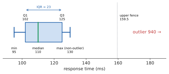
Worked example. Sorted: 95, 98, 102, 105, 108, 110, 115, 120, 125, 130, 940. Try it: Quartiles and box plot.
The 940 is far beyond 159.5: flagged. Nothing else is.
import statistics as st

times = [120, 95, 110, 130, 105, 98, 102, 115, 940, 108, 125]
print("mean  :", round(st.mean(times), 2))
print("median:", st.median(times))
print("stdev :", round(st.stdev(times), 2))      # sample sd, divides by n-1
trimmed = [t for t in times if t != 940]
print("without 940: mean", round(st.mean(trimmed), 2),
      "median", st.median(trimmed), "stdev", round(st.stdev(trimmed), 2))
print("quartiles (inclusive):", st.quantiles(times, n=4, method="inclusive"))
print("quartiles (exclusive):", st.quantiles(times, n=4))
mean : 186.18 median: 110 stdev : 250.25 without 940: mean 110.8 median 109.0 stdev 11.57 quartiles (inclusive): [103.5, 110.0, 122.5] quartiles (exclusive): [102.0, 110.0, 125.0]
Notice the last two lines: there are several conventions for quartiles, and software disagrees. For large data sets the differences vanish; for small ones, say which convention you used.
31.2.4. Box plots and histograms
A box plot draws the five-number summary: a box from \(Q_1\) to \(Q_3\) with a line at the median, "whiskers" out to the most extreme non-outlier values, and outliers as individual points.
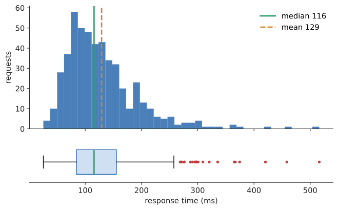
A histogram divides the range into bins and draws a bar for the count in each bin. It shows shape: one peak or two, symmetric or skewed, gaps, clusters. Box plots are compact and good for comparing many groups side by side; histograms show more detail about one group. Use both.
31.2.5. Skew
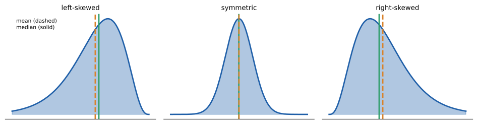
A distribution is right-skewed (positively skewed) if it has a long tail to the right: most values are moderate and a few are very large. Latencies, incomes, file sizes and city populations are right-skewed. Left-skewed is the mirror image (exam scores on an easy test). In a right-skewed distribution the mean is pulled into the tail, above the median; in a left-skewed one it’s below.
|
Outliers are information
Never delete an outlier just because the IQR rule flags it. Ask what produced it. A 940 ms request might be a measurement glitch (remove it, and say so) or the one user in a hundred who hits a cold cache (that’s the most important number on the dashboard). Report robust summaries (median, IQR, percentiles) and say how many outliers there were and what they were. For right-skewed data, the 1.5 × IQR rule flags many perfectly legitimate tail values, as in the box plot above. |
31.2.6. Where you’d use this
-
Everyday: house prices and pay. A street has nine houses worth £250,000 and one mansion worth £2.5 million. The mean value is \((9 \times 250\,000 + 2\,500\,000)/10 = 475\,000\) pounds, which describes no house on the street; the median, £250,000, describes nine of them. That’s why official statistics quote median house prices and median earnings.
-
Health: percentiles. A child "on the 75th percentile for height" is taller than 75% of children of the same age and sex. Growth charts are nothing but quantile curves, and a doctor watches for a child crossing several percentile lines, not for any single value.
-
Science and manufacturing: reporting spread. A lab result is written mean \(\pm\) standard deviation (or standard error, Section 31.4), and a factory tracks the standard deviation of a part’s diameter as closely as its mean: a machine can be perfectly centred and still produce scrap if its spread grows.
-
Sport: two basketball players both average 20 points a game; the one with the smaller standard deviation is the more predictable choice for a must-win game. The same comparison picks between two servers with equal median latency but different IQRs.
31.3. Samples, populations and bias
31.3.1. The problem
You want the average session length of all 40 million users, or the fraction of voters supporting a candidate, or the true conversion rate of a checkout page. You can’t measure everyone (or, for a conversion rate, "everyone" includes future users who don’t exist yet). You measure a sample and generalize. When is that legitimate, and how wrong might you be?
|
Population, sample, parameter, statistic
|
31.3.2. Bias: when samples lie
Random variation (noise) shrinks as samples grow. Bias doesn’t: it’s a systematic error that makes the sample unrepresentative no matter how large.
-
Selection bias. Surveying your users about your product says nothing about the people who left. Measuring latency only on successful requests ignores those that timed out, the slowest ones.
-
Survivorship bias. In the Second World War, analysts studied bullet holes in returning bombers and proposed armouring the most-hit areas. The statistician Abraham Wald pointed out that the planes hit in the other areas hadn’t returned: armour where the survivors had no holes.
-
Non-response bias. People who answer surveys differ from those who don’t.
-
Convenience samples. "The first 1,000 users who saw the new feature" are the most active, most engaged users, not typical ones.
|
The 1936 Literary Digest poll
In 1936 the Literary Digest mailed 10 million ballots, received 2.4 million back, and predicted a landslide for Alf Landon over Franklin Roosevelt. Roosevelt won 46 of 48 states. The mailing list came from telephone directories and car registrations, which in the Depression over-represented the wealthy, and those who replied were a self-selected group. George Gallup, with a sample of about 50,000 chosen to be representative, called the result correctly. A huge biased sample loses to a modest random one. |
|
Big data does not cure bias
Logs from millions of users feel like the whole population, but they are a sample of who used the product, in the way the product let them, while logging worked. The formulas in this chapter quantify random error only. They say nothing about bias, and a confidence interval around a biased estimate is a precise answer to the wrong question. The best cure is design: randomize who gets what (as in an A/B test) and sample at random rather than by convenience. |
31.4. Estimation and standard error
31.4.1. The problem
You sample 100 page loads and find a mean of 2.30 seconds. The true mean over all page loads is not exactly 2.30; a different sample of 100 would give a slightly different answer. How much would estimates bounce around from sample to sample?
31.4.2. Intuition: the sampling distribution
Imagine repeating the whole study many times, each time drawing a fresh sample of 100 and computing \(\bar x\). The collection of all those \(\bar x\) values has a distribution, the sampling distribution of the mean. Chapter 30 already told you its shape and size: by the central limit theorem it’s approximately normal, centred on the true \(\mu\), with standard deviation \(\sigma/\sqrt n\).
|
Standard error
The standard error (SE) of a statistic is the standard deviation of its sampling distribution: how much the statistic would vary from sample to sample.
Standard deviation describes the spread of individual data points; standard error describes the uncertainty of an estimate. Collecting more data doesn’t change the first and shrinks the second like \(1/\sqrt n\). |
If the 100 page loads have sample standard deviation \(s = 0.80\) s, then \(\text{SE} = 0.80/\sqrt{100} = 0.08\) s. Individual loads vary by about 0.8 s, but the average of 100 is uncertain by only about 0.08 s.
An estimator is unbiased if its sampling distribution is centred on the true parameter: \(E[\bar x] = \mu\), for instance. Good estimators are unbiased (or nearly) and have small standard errors.
31.5. Confidence intervals
31.5.1. The problem
"Average load time is 2.30 s" sounds more certain than it is. You want to report a range that honestly conveys the uncertainty, with a stated reliability.
31.5.2. Why it works
By the CLT, \(\bar x\) is approximately normal around \(\mu\) with standard deviation \(\text{SE}\). The 68–95–99.7 rule (more precisely, 95% lies within 1.96 standard deviations) says:
"\(\bar x\) is within 1.96 SE of \(\mu\)" is the same statement as "\(\mu\) is within 1.96 SE of \(\bar x\)". So
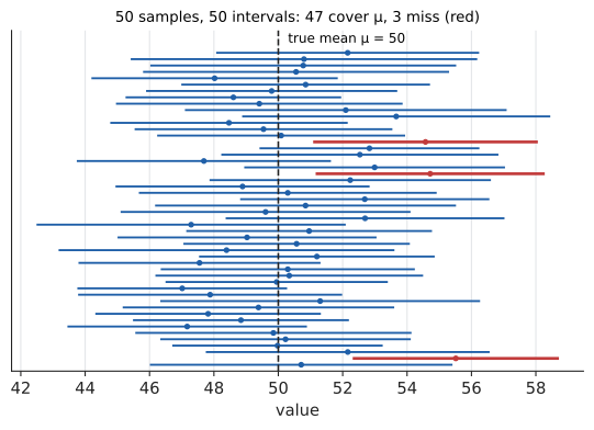
Read this carefully. \(\mu\) is a fixed (unknown) number; the randomness is in \(\bar x\), so in the interval. Before you collect data, the procedure "take \(\bar x \pm 1.96\,\text{SE}\)" has a 95% chance of producing an interval that captures \(\mu\).
|
Confidence interval
A 95% confidence interval for a parameter is an interval computed from the data by a procedure that captures the true parameter in 95% of repeated samples. For a mean:
\[\bar x \pm z^* \cdot \frac{s}{\sqrt n},\]
where \(z^* = 1.96\) for 95% (1.645 for 90%, 2.576 for 99%). The quantity \(z^* \cdot \text{SE}\) is the margin of error. The confidence level (95%) is the long-run success rate of the procedure. For small samples, replace \(z^*\) by a slightly larger \(t^*\) from the t-distribution (Section 31.6.6) to account for estimating \(\sigma\) by \(s\). |
Try it: When z* is too narrow.
Input: a random sample; a confidence level (say 95%).
Steps:
-
Compute the estimate: \(\bar x\) (mean) or \(\hat p\) (proportion).
-
Compute the standard error: \(s/\sqrt n\) or \(\sqrt{\hat p(1 - \hat p)/n}\).
-
Find the critical value: \(z^* = 1.96\) for 95% (or \(t^*\) with \(n - 1\) degrees of freedom for a small-sample mean).
-
Report estimate \(\pm\) critical value \(\times\) SE.
-
Check assumptions: random sample, independent observations, \(n\) large enough for the CLT (for proportions, at least about 10 successes and 10 failures).
Output: an interval and its confidence level.
Worked example. 100 page loads: \(\bar x = 2.30\) s, \(s = 0.80\) s.
Worked example (proportion). A poll of 1,000 randomly chosen users finds 540 prefer the new design.
That "±3 percentage points" is the margin of error quoted under news polls of about 1,000 people. To halve it, poll 4,000.
|
What a confidence interval does not mean
The common misreading is: "there is a 95% probability that \(\mu\) is between 2.14 and 2.46". In the frequentist framework that produced the interval, \(\mu\) is a fixed number, not a random one: it either is in \((2.14, 2.46)\) or it isn’t. The 95% describes the method: if you repeated the study many times, 95% of the intervals so produced would contain \(\mu\). The figure above is the picture to remember. Two other misreadings: a 95% CI does not contain 95% of the data (that would be roughly \(\bar x \pm 2s\), a much wider range), and it does not account for bias. If you want a statement like "95% probability that \(\mu\) lies here", that’s a Bayesian credible interval (Section 31.10), which requires a prior. |
Try it: Fifty intervals, live.
31.5.3. Where you’d use this
-
Physics: measuring \(g\). Ten timings of a pendulum give values of \(g\) with mean \(9.79\ \text{m/s}^2\) and \(s = 0.05\). Then \(\text{SE} = 0.05/\sqrt{10} \approx 0.016\), and with \(t^* = 2.262\) (9 degrees of freedom) the 95% interval is \(9.79 \pm 0.036 = (9.754, 9.826)\). The accepted value 9.81 is inside it, so the experiment agrees with theory. Every "result \(\pm\) uncertainty" in a physics or chemistry write-up is a confidence interval or a standard error.
-
Medicine: a trial reports that a drug lowers blood pressure by "8 mmHg (95% CI 5 to 11)". A doctor reads the lower end: even in the least favourable plausible case the benefit is 5 mmHg, which is clinically worthwhile.
-
Computing: benchmarks. Twenty runs of a benchmark average 412 ms with \(s = 30\) ms. The standard error is \(30/\sqrt{20} \approx 6.7\) ms and the 95% interval is \(412 \pm 2.093 \times 6.7 \approx 412 \pm 14\) ms. A claimed "3% speed-up" (about 12 ms) is inside that noise, so one run of each version proves nothing; report intervals, not single timings.
|
Catch the mean
Set a population (normal, skewed, or two-humped), a sample size and a confidence level, then press "sample" repeatedly. Each press draws a new sample and adds its interval to a growing stack, coloured by whether it covers the true mean. A counter shows the running coverage rate approaching the stated level, and a slider for \(n\) shows the intervals narrowing like \(1/\sqrt n\). A "biased sampling" switch shifts the population that samples come from, and coverage collapses even as intervals narrow. |
31.6. Hypothesis testing
31.6.1. The problem
A coin is tossed 100 times and lands heads 61 times. Is it biased? A fair coin could produce 61 heads; it would just be unusual. How unusual is unusual enough? The same question, with higher stakes: the new checkout page converted 11.0% of users versus 10.0% for the old one. Is the new page better, or did it get lucky?
31.6.2. Intuition: proof by contradiction, with probabilities
Hypothesis testing borrows the shape of proof by contradiction (Chapter 22). Assume the boring explanation, nothing is going on, and work out what data you’d expect. If the data you actually got would be very surprising under that assumption, you have evidence against it.
|
Hypotheses, test statistic, p-value, significance level
|
31.6.3. Worked example: the coin
\(H_0\): \(p = 0.5\). \(H_1\): \(p \ne 0.5\). Significance level \(\alpha = 0.05\). Try it: Run the z-test.
Under \(H_0\), the number of heads \(X \sim \text{Bin}(100, 0.5)\), with mean 50 and standard deviation \(\sqrt{100 \times 0.5 \times 0.5} = 5\).
Normal approximation. The test statistic is \(z = \frac{61 - 50}{5} = 2.2\). "At least as extreme, in either direction" means \(|Z| \ge 2.2\):
Exact binomial. Add the binomial probabilities of 61 or more heads and 39 or fewer: \(p \approx 0.035\). (The normal approximation is a little optimistic here; a "continuity correction" using 60.5 instead of 61 would bring it closer.)
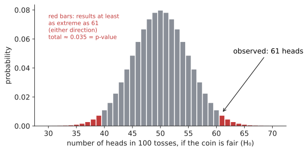
Either way \(p < 0.05\), so we reject \(H_0\) at the 5% level: 61 heads is evidence (moderate, not overwhelming) that the coin isn’t fair.
from math import comb, erf, sqrt

n, observed = 100, 61
pmf = [comb(n, k) / 2**n for k in range(n + 1)]
# two-sided: results at least as far from 50 as 61 is
p_exact = sum(p for k, p in enumerate(pmf) if abs(k - 50) >= abs(observed - 50))
z = (observed - 50) / 5
p_normal = 2 * (1 - 0.5 * (1 + erf(z / sqrt(2))))
print(round(p_exact, 4), round(z, 2), round(p_normal, 4))
0.0352 2.2 0.0278
Input: data; a question.
Steps:
-
State \(H_0\) and \(H_1\) in terms of a parameter. Choose \(\alpha\) before looking at the data.
-
Choose a test statistic and work out its distribution assuming \(H_0\) (the null distribution), by formula, normal approximation or simulation.
-
Compute the observed test statistic.
-
Compute the p-value: the probability under \(H_0\) of a statistic at least as extreme as observed (both tails for a two-sided \(H_1\)).
-
If \(p \le \alpha\), reject \(H_0\); otherwise fail to reject. Report the p-value and the estimated effect with a confidence interval.
Output: a decision, a p-value and an effect estimate.
31.6.4. What a p-value is, and what it isn’t
The p-value is \(P(\text{data this extreme} \mid H_0)\). Recall the warning from Chapter 29 about confusing \(P(A \mid B)\) with \(P(B \mid A)\).
-
It is not \(P(H_0 \mid \text{data})\), the probability that the null hypothesis is true. That’s the prosecutor’s fallacy again. To get \(P(H_0 \mid \text{data})\) you need Bayes' theorem and a prior: how plausible was \(H_0\) to begin with?
-
It is not the probability that the result is "due to chance".
-
It does not measure the size or importance of an effect. With a million users, a 0.01% improvement can have \(p < 0.001\) and be worthless; with 20 users, a huge improvement can have \(p = 0.2\).
-
\(p > 0.05\) does not show that \(H_0\) is true. "Fail to reject" means "not enough evidence", not "evidence of no effect". Absence of evidence is not evidence of absence, especially in a small study.
-
The 0.05 threshold is a convention (from R. A. Fisher in the 1920s), not a law of nature. \(p = 0.049\) and \(p = 0.051\) are essentially the same evidence.
31.6.5. Type I and type II errors, and power
A test makes a binary decision about an unknown truth, so it can be wrong in two ways:
| \(H_0\) true (no effect) | \(H_0\) false (real effect) | |
|---|---|---|
Reject \(H_0\) |
Type I error (false positive). Probability \(\alpha\). |
Correct: a true discovery. Probability = power. |
Fail to reject |
Correct. |
Type II error (false negative). Probability \(\beta\). |
|
Type I and type II errors, power
Power increases with larger samples, larger true effects, less noisy data, and a larger \(\alpha\). For a fixed sample size, lowering \(\alpha\) (fewer false alarms) raises \(\beta\) (more misses). |
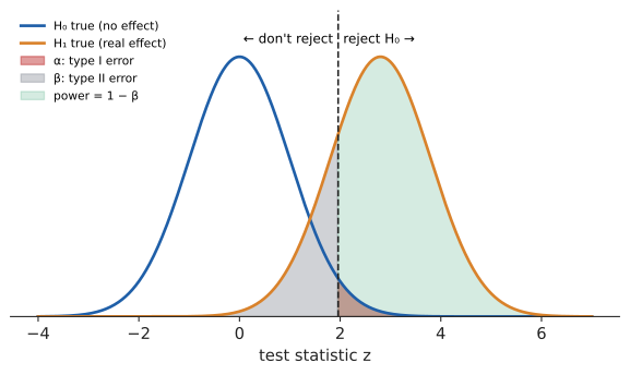
The analogy is a smoke alarm. Make it more sensitive and it catches more fires (more power) but also goes off for toast (more type I errors). The only way to improve both is a better detector, which in statistics means more data or less noise.
|
Underpowered studies
An experiment with too little data is worse than useless. It usually fails to find a real effect, and when it does reach significance, it’s typically because noise exaggerated the effect: significant results from low-powered studies systematically overestimate effect sizes (the "winner’s curse"). Work out the sample size you need before running the experiment (Section 31.11). |
31.6.6. Comparing two means: the t-test, intuitively
The problem. A new build’s latencies (8 runs, ms): 190, 204, 185, 199, 210, 188, 195, 202. The old build: 212, 198, 225, 240, 205, 219, 230, 201. Means 196.6 and 216.3, a difference of 19.6 ms. Real, or noise? Try it: Run Welch’s t-test.
The idea. Every two-sample test asks the same thing: is the difference between groups large compared with how much it would vary by chance? The t statistic is
The denominator combines the standard errors of the two means (variances of independent quantities add, Chapter 30). Here \(t \approx 3.23\): the observed difference is more than three standard errors from zero.
Why "t" and not "z"? With small samples, \(s\) is itself a noisy estimate of \(\sigma\), which adds uncertainty. William Gosset worked out the exact null distribution of \(t\) for normal data in 1908: the t-distribution, a bell curve with heavier tails than the normal, controlled by the degrees of freedom (roughly \(n - 1\) per group). Some 95% two-sided critical values:
| degrees of freedom | 5 | 10 | 11 | 30 | \(\infty\) |
|---|---|---|---|---|---|
\(t^*\) |
2.571 |
2.228 |
2.201 |
2.042 |
1.960 |
Welch’s formula for unequal variances gives about 11 degrees of freedom here, and \(|t| = 3.23 > 2.201\), so the difference is significant at the 5% level. As \(n\) grows, \(t^*\) approaches the normal’s 1.96.
An alternative that needs no tables: the permutation test. If the build made no difference (\(H_0\)), the labels "old" and "new" are arbitrary: any 8 of the 16 numbers could equally have been the "old" ones. So shuffle the labels thousands of times, recompute \(t\) each time, and see how often a shuffle gives a result as extreme as the real one. That fraction is the p-value, computed directly from its definition. Try it: Permutation test vs t-test.
import random, statistics as st

old = [212, 198, 225, 240, 205, 219, 230, 201]   # ms, old build
new = [190, 204, 185, 199, 210, 188, 195, 202]   # ms, new build

def welch_t(a, b):
    se = (st.variance(a) / len(a) + st.variance(b) / len(b)) ** 0.5
    return (st.mean(a) - st.mean(b)) / se

t_obs = welch_t(old, new)
print("difference in means:", st.mean(old) - st.mean(new))
print("t =", round(t_obs, 3))

# Permutation test: if the build made no difference, labels are arbitrary.
rng = random.Random(13)
pooled = old + new
trials, extreme = 20_000, 0
for _ in range(trials):
    rng.shuffle(pooled)
    if abs(welch_t(pooled[:8], pooled[8:])) >= abs(t_obs):
        extreme += 1
print("permutation p-value ~", round(extreme / trials, 4))
Try it: Run this in your browser.
difference in means: 19.625
t = 3.227
permutation p-value ~ 0.0067
Choosing a method. Use a t-test for comparing means when data are roughly normal or samples are moderately large; it’s standard and fast. Use a permutation test when samples are small and skewed, or for any statistic (medians, ratios) without a textbook formula; it costs only computer time. For paired data (the same 8 benchmarks run on both builds) use a paired test on the differences, which removes benchmark-to-benchmark variation and is far more powerful.
|
Student’s t and Guinness
William Sealy Gosset was a chemist at the Guinness brewery in Dublin, testing barley and hops with small samples. Guinness forbade employees from publishing (a rival had leaked trade secrets), so he published his 1908 paper under the pseudonym "Student". The t-test is still called "Student’s t-test", a brewery quality-control method that became one of the most used tools in science. |
31.6.7. Counts in categories: the chi-squared test, briefly
For categorical data, compare observed counts with the counts expected under \(H_0\). A die is rolled 120 times; if fair, each face is expected 20 times. Observed: 15, 22, 18, 25, 17, 23. The chi-squared statistic sums the squared discrepancies, each scaled by its expected count: Try it: Run the χ² test.
(\(\chi\) is the Greek letter chi, pronounced "kai".) Under \(H_0\) this statistic follows a chi-squared distribution with \(6 - 1 = 5\) degrees of freedom, whose 95% critical value is 11.07. Since \(3.8 < 11.07\), there’s no evidence the die is unfair; deviations this size are routine. The same test checks whether two categorical variables are independent in a two-way table (does the browser affect whether checkout succeeds?), and whether a random number generator or hash function spreads values evenly across buckets.
31.6.8. Where you’d use this
-
Biology: Mendel’s peas. Mendel’s genetics predicts round and wrinkled seeds in a 3 : 1 ratio. Of 7,324 seeds he counted 5,474 round and 1,850 wrinkled; the expected counts are 5,493 and 1,831. Then \(\chi^2 = \frac{19^2}{5493} + \frac{19^2}{1831} \approx 0.26\), far below the 1-degree-of-freedom critical value 3.84: the data fit the theory. (Fisher later argued that Mendel’s results overall fit too well, a statistical accusation of tidying the data.)
-
Medicine: every new drug must beat a placebo in a randomized trial at a pre-agreed significance level (typically two-sided \(\alpha = 0.05\)) with a pre-computed sample size giving 80–90% power. The type I error is approving a useless drug; the type II error is abandoning a useful one.
-
Everyday: "hot streaks". A basketball player who usually makes 50% of shots makes 8 in a row. Is that evidence of a hot hand? For one specific run of 8 shots, \(P = 0.5^8 \approx 0.004\); but a player takes hundreds of shots a season, so a run of 8 somewhere is not surprising at all. Whether a "streak" is significant depends on how many chances it had to happen (Section 31.9).
-
Computing: catching performance regressions. Continuous-integration systems run each benchmark several times on the old and new commit and apply a t-test or permutation test; only differences with a small p-value and a meaningful size raise an alert, which keeps noisy benchmarks from crying wolf on every commit.
31.7. Correlation, causation and Simpson’s paradox
31.7.1. Correlation is not causation
Chapter 30 defined the correlation coefficient. For data pairs \((x_i, y_i)\), the sample correlation is
a number from \(-1\) to 1 measuring the strength of a linear association. Ice-cream sales correlate with drownings. Countries' chocolate consumption correlates with Nobel prizes per capita. Users who enable dark mode have higher retention. None of these shows that one thing causes the other. The usual explanations are:
-
Confounding: a third variable drives both. Hot weather causes both ice-cream sales and swimming; engaged users both find settings like dark mode and stay longer.
-
Reverse causation: \(Y\) causes \(X\). Do happy users write reviews, or does writing reviews make users happy?
-
Selection: the sample was filtered in a way that creates a relationship.
-
Chance: with enough variables, some will correlate by luck (Section 31.9).
The gold standard for causation is a randomized controlled experiment: assign the treatment at random, so that confounders are balanced between groups on average. That’s exactly what an A/B test does, and why it can answer causal questions that no amount of observational log analysis can.
31.7.2. Simpson’s paradox
A 1986 study compared two treatments for kidney stones: Try it: Slide through Simpson’s paradox.
| Treatment A | Treatment B | |
|---|---|---|
Small stones |
81/87 = 93% |
234/270 = 87% |
Large stones |
192/263 = 73% |
55/80 = 69% |
All patients |
273/350 = 78% |
289/350 = 83% |
Treatment A is better for small stones and better for large stones, yet B looks better overall. How?
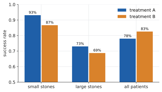
Look at who got which treatment. Treatment A was given mostly to large stones (263 of 350), the hard cases; B mostly to small stones (270 of 350), the easy ones. The overall rate is a weighted average of the group rates (the law of total probability from Chapter 29), and the weights differ: A’s average is dominated by its 73% group, B’s by its 87% group. Stone size is a confounder: it affects both which treatment doctors chose and the chance of success. Try it: Same case mix, no paradox.
The right comparison here is within groups: A is better. But Simpson’s paradox doesn’t come with a rule that "always disaggregate"; which comparison is right depends on the causal story. If the grouping variable were itself caused by the treatment, aggregating would be correct.
|
Spotting Simpson’s paradox in product data
"Conversion fell after the redesign" might be entirely because the mix of traffic changed (more mobile users, who always convert less), while conversion rose within every platform. Whenever group sizes differ between the things you compare, break the comparison down by the obvious grouping variables (platform, country, new versus returning) before concluding anything. Randomization protects A/B tests from this, because it makes the mix the same in both arms on average. |
31.8. Simple linear regression
31.8.1. The problem
A service’s median response time at six load levels (load in hundreds of concurrent users):
| load \(x\) | 1 | 2 | 3 | 4 | 5 | 6 |
|---|---|---|---|---|---|---|
response \(y\) (ms) |
51 |
52 |
59 |
63 |
64 |
71 |
Response time clearly grows with load. You want a line through the data to summarize the trend and predict, say, the response at load 8. The points don’t lie exactly on any line, so which line is "best"?
31.8.2. Intuition: least squares
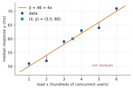
For any candidate line \(\hat y = a + bx\), each point has a residual: the vertical miss \(e_i = y_i - \hat y_i\) (observed minus predicted). A good line makes residuals small. The least-squares line makes the sum of squared residuals as small as possible. Squaring treats overshoots and undershoots alike, punishes big misses heavily, and (the decisive practical reason) gives a clean formula.
|
Least squares regression line and residuals
The least-squares regression line (or line of best fit) of \(y\) on \(x\) is \(\hat y = a + bx\) with
\[b = \frac{S_{xy}}{S_{xx}} = \frac{\sum (x_i - \bar x)(y_i - \bar y)}{\sum (x_i - \bar x)^2}, \qquad a = \bar y - b\,\bar x.\]
\(b\) is the slope (change in predicted \(y\) per unit of \(x\)); \(a\) is the intercept. The line always passes through the point of means \((\bar x, \bar y)\). \(\hat y\) ("y-hat") denotes a predicted value. A residual is \(y_i - \hat y_i\). |
31.8.3. Why it works (light derivation)
Write the total squared error as \(\text{SSE}(a, b) = \sum (y_i - a - bx_i)^2\). Two observations give the formulas.
The intercept. For a fixed slope \(b\), SSE is the sum of squared distances from the numbers \(y_i - bx_i\) to a single number \(a\). The number that minimizes a sum of squared distances is the mean (you can verify this by completing the square, Chapter 8): \(a = \overline{y - bx} = \bar y - b\bar x\). So the best line passes through \((\bar x, \bar y)\).
The slope. Substitute \(a = \bar y - b\bar x\) and write \(X_i = x_i - \bar x\), \(Y_i = y_i - \bar y\) (centred data). Then \(\text{SSE}(b) = \sum (Y_i - bX_i)^2 = S_{yy} - 2bS_{xy} + b^2 S_{xx}\), a quadratic in \(b\) that opens upward. Its vertex (Chapter 8) is at \(b = S_{xy}/S_{xx}\).
(Optional, with calculus: setting \(\partial\,\text{SSE}/\partial a = 0\) and \(\partial\,\text{SSE}/\partial b = 0\) gives the same two equations, the normal equations; see Chapter 20. With many input variables they become the matrix equation of Section 33.2.)
31.8.4. Worked example
\(\bar x = 21/6 = 3.5\) and \(\bar y = 360/6 = 60\). Try it: Fit the load data; Fit the regression line.
| \(x\) | \(y\) | \(x - \bar x\) | \(y - \bar y\) | \((x - \bar x)(y - \bar y)\) | \((x - \bar x)^2\) |
|---|---|---|---|---|---|
1 |
51 |
\(-2.5\) |
\(-9\) |
22.5 |
6.25 |
2 |
52 |
\(-1.5\) |
\(-8\) |
12 |
2.25 |
3 |
59 |
\(-0.5\) |
\(-1\) |
0.5 |
0.25 |
4 |
63 |
0.5 |
3 |
1.5 |
0.25 |
5 |
64 |
1.5 |
4 |
6 |
2.25 |
6 |
71 |
2.5 |
11 |
27.5 |
6.25 |
Sum |
\(S_{xy} = 70\) |
\(S_{xx} = 17.5\) |
Each extra 100 concurrent users adds about 4 ms. The prediction at load 8 is \(46 + 32 = 78\) ms, an extrapolation beyond the data, to be trusted only if the trend stays linear (queueing theory says it won’t near saturation; see the Watch out below).
31.8.5. How good is the fit? \(R^2\)
Compare the line’s errors with the errors of the dumbest prediction, "always predict \(\bar y\)":
Here the residuals are \(51 - 50 = 1\), \(52 - 54 = -2\), \(59 - 58 = 1\), \(63 - 62 = 1\), \(64 - 66 = -2\), \(71 - 70 = 1\), so \(\text{SS}_{\text{res}} = 1 + 4 + 1 + 1 + 4 + 1 = 12\). And \(\text{SS}_{\text{tot}} = 81 + 64 + 1 + 9 + 16 + 121 = 292\). So
The line explains about 96% of the variation in response time. For simple linear regression, \(R^2 = r^2\), so \(r = \sqrt{0.959} \approx 0.979\).
def least_squares(xs, ys):
    n = len(xs)
    xbar, ybar = sum(xs) / n, sum(ys) / n
    sxy = sum((x - xbar) * (y - ybar) for x, y in zip(xs, ys))
    sxx = sum((x - xbar) ** 2 for x in xs)
    b = sxy / sxx
    a = ybar - b * xbar
    ss_res = sum((y - (a + b * x)) ** 2 for x, y in zip(xs, ys))
    ss_tot = sum((y - ybar) ** 2 for y in ys)
    return a, b, 1 - ss_res / ss_tot

a, b, r2 = least_squares([1, 2, 3, 4, 5, 6], [51, 52, 59, 63, 64, 71])
print(a, b, round(r2, 4))
46.0 4.0 0.9589
|
Regression pitfalls
|
31.8.6. Where you’d use this
-
Physics: Hooke’s law. Hang loads of 1, 2, 3, 4, 5 N on a spring and measure extensions 2.1, 3.9, 6.2, 7.8, 10.1 mm. The least-squares line is \(\hat y = 0.05 + 1.99x\), so the spring stretches about 1.99 mm per newton and its spring constant is \(k \approx 1/1.99 \approx 0.50\) N/mm (about 500 N/m). The intercept near 0 is a check that the law holds; the slope is the physical constant you wanted. Calibration curves in chemistry (absorbance against concentration) work the same way.
-
Everyday and finance: fit your monthly fuel cost against miles driven, and the slope is your cost per mile while the intercept is what you’d spend standing still. In finance, a stock’s beta is the regression slope of its returns on the market’s returns: beta 1.5 means it tends to move 1.5% when the market moves 1%.
-
Computing: measuring complexity. A function takes 0.012, 0.049, 0.19 and 0.78 s on inputs of size 1,000, 2,000, 4,000 and 8,000. Regress \(\ln(\text{time})\) on \(\ln n\) (if time \(\approx c\,n^k\), then \(\ln \text{time} = \ln c + k \ln n\), a straight line); the slope comes out at 2.0, so the algorithm is quadratic and 100,000 items will take about \(0.78 \times 12.5^2 \approx 120\) s. Fitting straight lines to transformed data is how you read growth rates from measurements (Chapter 12).
31.9. Multiple comparisons
31.9.1. The problem
You run an A/B test and check 20 metrics: conversion, revenue, clicks, time on page, each on mobile and desktop, in five countries. One metric shows \(p = 0.03\). Discovery?
31.9.2. Why it’s a problem
At \(\alpha = 0.05\), each test of a true null has a 5% chance of a false positive. With 20 independent tests of true nulls, Try it: Simulate twenty tests.
You’re more likely than not to find "something", even if the change did nothing. Testing many hypotheses and reporting the significant ones is called p-hacking or data dredging, and is a central cause of the replication crisis in psychology, medicine and other fields: many published "findings" were simply the lucky tail of many tries. The same thing happens if you test one hypothesis but try many analyses (different outlier rules, different subgroups, different stopping times) and report the one that worked.
31.9.3. Remedies
-
Pre-register. Decide on one primary metric and the analysis before collecting data; treat the rest as exploratory, to be confirmed in a new experiment.
-
Bonferroni correction. With \(m\) tests, use threshold \(\alpha/m\) for each (0.0025 for 20 tests). This bounds the chance of any false positive by \(\alpha\). Simple and conservative (it loses power). Try it: Bonferroni in action.
-
False discovery rate (FDR) control, such as the Benjamini–Hochberg procedure, bounds the expected fraction of false positives among the discoveries instead. Better when you’re screening many candidates (genes, features, metrics). Try it: Benjamini–Hochberg on 100 tests.
|
The dead salmon
In 2009 neuroscientists put a dead Atlantic salmon in an fMRI scanner, showed it photographs of people in social situations, and "asked" it to judge their emotions. Analysing tens of thousands of brain voxels without a multiple-comparisons correction, they found a cluster of "significant" activity in the fish’s brain. The poster won an Ig Nobel Prize, and the point landed: with enough tests, noise always produces significance somewhere. |
31.10. Bayesian and frequentist perspectives
Everything above is frequentist: probabilities describe long-run frequencies over repeated samples, parameters are fixed unknowns, and procedures (intervals, tests) are judged by how often they’d be right. That’s why a confidence interval’s 95% describes the procedure, and why a p-value conditions on \(H_0\) rather than computing its probability.
The Bayesian approach (from Chapter 29's degree-of-belief interpretation) treats an unknown parameter as uncertain and describes that uncertainty with a probability distribution. Start with a prior distribution, observe data, and use Bayes' theorem to get the posterior:
where \(\theta\) (theta) is the parameter and \(\propto\) means "proportional to" (the denominator just rescales so the posterior has total probability 1). Then you can say directly: "there is a 95% probability that \(\theta\) is in this range" (a credible interval), or "there’s a 99.8% probability that version B converts better than A".
| Frequentist | Bayesian | |
|---|---|---|
Parameter |
fixed, unknown |
uncertain, has a distribution |
Probability means |
long-run frequency |
degree of belief |
Answers |
"how surprising is this data if \(H_0\) holds?" (p-value) |
"how probable is the hypothesis, given the data?" (posterior) |
Needs |
a sampling model |
a sampling model and a prior |
Strengths |
no prior to argue about; well-understood error rates |
direct, intuitive answers; combines evidence naturally; good with small data |
Weaknesses |
answers are easy to misread |
results depend on the prior; computation can be heavy |
In practice, with plenty of data and a mild prior, the two approaches give nearly the same numbers; they differ in interpretation and in small-data situations. Many practitioners use both: frequentist error control for decisions that must be defensible, Bayesian models where prior knowledge is real and direct probability statements are wanted. A Bayesian treatment of the A/B test follows in the next section.
31.11. A/B testing, end to end
31.11.1. The problem
Your checkout page converts 10% of visitors. A redesign might help. You’ll randomly show half of new visitors the old page (A, control) and half the new one (B, treatment). How many visitors do you need, how do you analyse the result, and what mistakes must you avoid?
31.11.2. Step 1: decide what you’re testing, before you start
-
Primary metric: conversion rate (fraction of visitors who purchase).
-
Hypotheses: \(H_0: p_B = p_A\); \(H_1: p_B \ne p_A\) (two-sided, so you’d also detect harm).
-
\(\alpha = 0.05\), power 80%.
-
Minimum detectable effect (MDE): the smallest improvement worth detecting. Say 1 percentage point (10% to 11%). Smaller effects exist, but you’ve decided they’re not worth the engineering cost, or not worth the time to detect.
31.11.3. Step 2: sample size
The test statistic is the difference in sample proportions divided by its standard error. For the test to have power 80%, the true difference must be large enough that the test statistic’s distribution under \(H_1\) sits mostly beyond the cut-off 1.96 (the figure in the type I/II section). The standard approximation is Try it: Plan the sample size.
where \(z_{\alpha/2} = 1.96\) (two-sided 5%) and \(z_\beta = 0.84\) (\(\Phi(0.84) \approx 0.80\), for 80% power). With \(p_A = 0.10\), \(p_B = 0.11\):
About 30,000 visitors in total. Note the denominator: the required sample grows with the inverse square of the effect. Detecting a 0.5-point lift needs about four times as many users (roughly 58,000 per group); a 0.1-point lift, a hundred times as many. Try it: Half-point lift sample size.
31.11.4. Step 3: run it properly
-
Randomize at the right unit (usually the user, not the page view, so the same person sees a consistent version), using a hash of the user ID.
-
Run for the planned sample size, and for whole weeks to average over weekly cycles.
-
Don’t peek and stop early (see the simulation below).
-
Check the split: if you intended 50/50 and got 50.8/49.2 on 30,000 users, a chi-squared test will flag a sample ratio mismatch, which usually means a bug in assignment or logging, and invalidates the test.
31.11.5. Step 4: analyse
Results: A converted 1,500 of 15,000 (10.0%); B converted 1,650 of 15,000 (11.0%). Try it: Run the two-proportion test.
Significant at the 5% level. For the confidence interval, use the unpooled standard error (we no longer assume the rates are equal):
Report: "B increased conversion by 1.0 percentage point (95% CI 0.3 to 1.7 points; \(p = 0.005\))." The interval matters as much as the p-value: the true lift could plausibly be as small as 0.3 points. Is that still worth shipping? That’s a business decision the statistics informs but doesn’t make.
from math import erf, sqrt

def phi(z):
    return 0.5 * (1 + erf(z / sqrt(2)))

def ab_test(conv_a, n_a, conv_b, n_b):
    pa, pb = conv_a / n_a, conv_b / n_b
    pooled = (conv_a + conv_b) / (n_a + n_b)
    se0 = sqrt(pooled * (1 - pooled) * (1 / n_a + 1 / n_b))   # under H0
    z = (pb - pa) / se0
    p_value = 2 * (1 - phi(abs(z)))
    se = sqrt(pa * (1 - pa) / n_a + pb * (1 - pb) / n_b)      # for the CI
    ci = (pb - pa - 1.96 * se, pb - pa + 1.96 * se)
    return z, p_value, ci

z, p, ci = ab_test(1500, 15_000, 1650, 15_000)
print(f"z = {z:.2f}, p = {p:.4f}, 95% CI for lift = "
      f"({ci[0]*100:.2f}, {ci[1]*100:.2f}) percentage points")

def sample_size(p1, p2, z_alpha=1.96, z_beta=0.8416):
    return (z_alpha + z_beta) ** 2 * (p1 * (1 - p1) + p2 * (1 - p2)) / (p2 - p1) ** 2

print(round(sample_size(0.10, 0.11)))
z = 2.83, p = 0.0047, 95% CI for lift = (0.31, 1.69) percentage points 14748
31.11.6. Step 5: check the whole procedure by simulation
Does the procedure really have a 5% false-positive rate and 80% power? And what does peeking do? Simulate thousands of experiments where you know the truth.
import numpy as np

rng = np.random.default_rng(14)
n, experiments = 15_000, 20_000

def z_stats(conv_a, conv_b, n):
    pooled = (conv_a + conv_b) / (2 * n)
    se = np.sqrt(pooled * (1 - pooled) * 2 / n)
    return (conv_b - conv_a) / n / se

# A/A tests: both arms truly convert at 10%
a = rng.binomial(n, 0.10, experiments)
b = rng.binomial(n, 0.10, experiments)
print("false positive rate:", np.mean(np.abs(z_stats(a, b, n)) > 1.96))

# A/B tests: B truly converts at 11%
b = rng.binomial(n, 0.11, experiments)
print("power              :", np.mean(np.abs(z_stats(a, b, n)) > 1.96))

# Peeking: check after every 1,000 users per arm, stop at first "significant" result
checks = np.arange(1000, n + 1, 1000)
stopped = 0
for _ in range(2000):
    xa = rng.random(n) < 0.10
    xb = rng.random(n) < 0.10            # no real difference
    ca, cb = np.cumsum(xa)[checks - 1], np.cumsum(xb)[checks - 1]
    pooled = (ca + cb) / (2 * checks)
    z = (cb - ca) / checks / np.sqrt(pooled * (1 - pooled) * 2 / checks)
    stopped += np.any(np.abs(z) > 1.96)
print("false positive rate with peeking:", stopped / 2000)false positive rate: 0.04755 power : 0.80715 false positive rate with peeking: 0.2265
The planned test behaves as designed: about 5% false positives when nothing changed, about 80% detection of a real 1-point lift. But checking 15 times and stopping at the first significant result raises the false-positive rate from 5% to about 23%. Each look is another chance for noise to cross the line: a multiple-comparisons problem in time. If you need to monitor continuously, use methods designed for it (sequential tests, or "always-valid" p-values), which set stricter thresholds for early looks.
31.11.7. A Bayesian reading of the same data
With a uniform prior on each conversion rate, the posterior for a rate after \(s\) successes and \(f\) failures is a Beta distribution, Beta(\(s + 1, f + 1\)). Sampling from both posteriors answers the question stakeholders actually ask:
import numpy as np

rng = np.random.default_rng(15)
# Uniform prior on each conversion rate -> Beta(conversions+1, failures+1) posterior
post_a = rng.beta(1500 + 1, 13_500 + 1, 200_000)
post_b = rng.beta(1650 + 1, 13_350 + 1, 200_000)
print("P(B better than A) =", round(np.mean(post_b > post_a), 4))
print("P(lift > 0.5 points) =", round(np.mean(post_b - post_a > 0.005), 3))
P(B better than A) = 0.9978 P(lift > 0.5 points) = 0.921
"There’s a 99.8% probability B is better, and a 92% probability the lift exceeds half a point", given the model and the (flat) prior. With this much data the prior barely matters, and the conclusions agree with the frequentist analysis.
|
A/B testing failure modes
|
|
Plan an experiment
Sliders for baseline rate, minimum detectable effect, \(\alpha\) and power compute the required sample size live, with a plot of the two sampling distributions (null and alternative) moving apart as \(n\) grows. A "run" button simulates the experiment day by day, showing the z-score’s random walk and the 1.96 boundary; a "peek" toggle lets you stop at the first crossing, while a counter over many replays shows the false-positive rate climbing. Try it: Plan an experiment |
Try it: Watch the bootstrap resample. === The bootstrap
31.11.8. The problem
You have 200 response times and want a confidence interval for the median, or the p99, or the ratio of two medians. There’s no simple standard-error formula like \(s/\sqrt n\) for these. The sampling distribution you need comes from imagining many repeated samples from the population, but you only have one sample.
31.11.9. Intuition: resample your sample
Your sample is your best picture of the population. So treat it as the population: draw a new sample of the same size from it, with replacement (some values appear twice, some not at all), and compute the statistic. Repeat thousands of times. The spread of these bootstrap statistics approximates the spread of the statistic across real repeated samples.
The name comes from the impossible feat of "pulling yourself up by your bootstraps". It does feel like getting something for nothing, but it works remarkably well when the sample is reasonably large and representative.
Input: a sample \(x_1, \ldots, x_n\); a statistic (median, p99, …); a number of resamples \(B\) (e.g. 5,000); a level (e.g. 95%).
Steps:
-
Compute the statistic on the original sample: the estimate.
-
Repeat \(B\) times: draw \(n\) values from the sample uniformly with replacement; compute the statistic on this resample; store it.
-
Sort the \(B\) stored values. The 2.5th and 97.5th percentiles are the ends of the 95% interval.
-
Look at the histogram of the stored values: a lumpy or very skewed shape is a warning.
Output: the estimate and a bootstrap confidence interval.
import numpy as np

def bootstrap_ci(data, stat=np.median, resamples=5000, level=0.95, seed=0):
    rng = np.random.default_rng(seed)
    data = np.asarray(data)
    stats = np.array([stat(rng.choice(data, size=data.size, replace=True))
                      for _ in range(resamples)])
    tail = (1 - level) / 2 * 100
    return stat(data), np.percentile(stats, [tail, 100 - tail])

rng = np.random.default_rng(2024)
latencies = rng.lognormal(mean=np.log(120), sigma=0.6, size=200)  # stand-in data
est, (lo, hi) = bootstrap_ci(latencies, seed=1)
print(f"median = {est:.1f} ms, 95% bootstrap CI = ({lo:.1f}, {hi:.1f})")
est, (lo, hi) = bootstrap_ci(latencies, stat=lambda x: np.percentile(x, 99), seed=1)
print(f"p99    = {est:.1f} ms, 95% bootstrap CI = ({lo:.1f}, {hi:.1f})")
median = 121.8 ms, 95% bootstrap CI = (109.8, 132.4) p99 = 462.8 ms, 95% bootstrap CI = (371.7, 511.1)
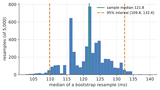
The p99 interval is wide and lopsided: with 200 data points, only the top two values inform the 99th percentile, so it is very uncertain. That’s useful knowledge before anyone alerts on a p99 from a small window of requests. Try it: Bootstrap the p99.
Choosing a method. Use formula-based intervals for means and proportions with decent sample sizes: they’re exact enough and instant. Use the bootstrap for medians, percentiles, ratios, correlations, model-evaluation metrics, or anything complicated. The bootstrap struggles for extreme statistics (maximum, very high percentiles with small samples), for very small samples, and for dependent data (time series need block resampling).
|
Bradley Efron’s computer-age statistics
Bradley Efron introduced the bootstrap in 1979. It replaced pages of approximate algebra with brute-force computation, and was initially regarded with suspicion for exactly that reason. It is now one of the most used methods in applied statistics, and Efron received the inaugural International Prize in Statistics in 2016 for it. It’s a clear case where cheap computing changed which mathematics was practical. |
31.12. Evaluating classifiers and search: precision, recall, F1
31.12.1. The problem
A fraud model flags transactions; a search engine returns documents; a spam filter sends email to junk. How good are they? "Accuracy" (fraction of correct decisions) is often useless: if 1% of transactions are fraudulent, a model that never flags anything is 99% accurate. You need measures that focus on the class you care about.
31.12.2. The confusion matrix
Every decision lands in one of four cells:
| Actually positive | Actually negative | |
|---|---|---|
Predicted positive |
True positive (TP) |
False positive (FP) |
Predicted negative |
False negative (FN) |
True negative (TN) |
|
Precision, recall, F1
In probability language (Chapter 29): recall is \(P(\text{flagged} \mid \text{positive})\) and precision is \(P(\text{positive} \mid \text{flagged})\), the two directions of conditioning. Precision is the medical test’s "probability of disease given a positive test", and so it depends on the base rate. |
Worked example: search. A query has 30 relevant documents in the collection. The engine returns 20 results, of which 12 are relevant.
Worked example: a rare-class classifier. A fraud model on 10,000 transactions, 100 of them fraudulent, catches 90 frauds and wrongly flags 150 legitimate transactions. Recall \(= 90/100 = 0.90\); precision \(= 90/240 = 0.375\); F1 \(\approx 0.53\). Accuracy \(= (90 + 9\,750)/10\,000 = 98.4\%\), which sounds great and tells you almost nothing; it’s lower than the 99% of the do-nothing model. Try it: Precision, recall and F1.
def precision_recall_f1(tp, fp, fn):
    precision = tp / (tp + fp)
    recall = tp / (tp + fn)
    f1 = 2 * precision * recall / (precision + recall)
    return precision, recall, f1

print(precision_recall_f1(tp=12, fp=8, fn=18))     # search example
print(precision_recall_f1(tp=90, fp=150, fn=10))   # rare-class classifier
Try it: Run this in your browser.
(0.6, 0.4, 0.48)
(0.375, 0.9, 0.5294117647058825)
31.12.3. The tradeoff
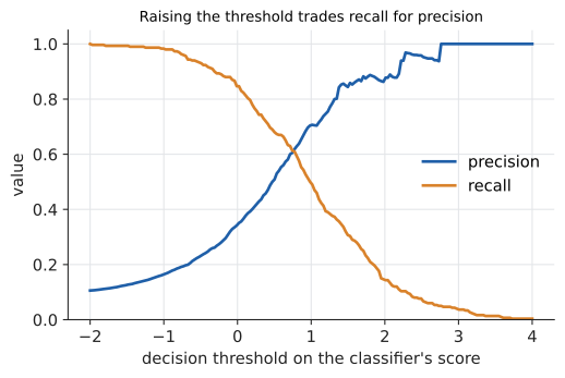
Most classifiers output a score, and you choose a threshold. Lower the threshold and you flag more: recall rises, precision usually falls. Raise it and the reverse happens. Which balance is right depends on the costs. Missing fraud is expensive, so favour recall; showing users junk results in the top 10 is expensive, so favour precision. Try it: Move the threshold.
|
Precision, recall and the base rate
Recall and the false-positive rate are properties of the classifier; precision also depends on how common positives are. A model evaluated on a balanced test set (50% fraud) will show far higher precision than it achieves in production (1% fraud). Always evaluate on data with the real-world class balance, or recompute precision with Bayes' theorem for the production base rate. |
31.12.4. Where you’d use this
-
Health: home tests. A rapid antigen test with recall (sensitivity) 80% and a false-positive rate of 0.5% is used when 1% of people are infected. Per 10,000 people: 100 infected, 80 test positive; 9,900 not infected, about 50 test positive. Precision is \(80/130 \approx 0.62\): more than a third of positive results are false, which is why positives were often confirmed by a lab test. Meanwhile 20 of the 100 infected people get a reassuring negative: low recall is why a negative test was never a free pass.
-
Everyday: airport security and smoke alarms are tuned for recall (missing a weapon or a fire is catastrophic) and accept poor precision (most bag searches and alarms are false). A music app’s "you might like" list is tuned the other way: a few bad suggestions annoy, a missed song costs nothing.
31.13. Interactive tools
Browser tools on the companion website that go with this chapter. Each example link in the chapter opens one of them with that example already set up.
31.14. Exercises
-
(Recognition) For each, say whether the mean or the median is the better summary of "typical", and why: (a) household incomes in a city; (b) heights of adult women; (c) time users spend on a page; (d) the number of bugs per 1,000 lines in a well-tested codebase.
-
(Recognition) Classify each as type I error, type II error or correct decision: (a) an A/B test declares a useless change "significant"; (b) a smoke alarm stays silent during a fire; (c) a test fails to find an effect that doesn’t exist.
-
(Application) Find the five-number summary, IQR and any outliers (1.5 × IQR rule) for: 3, 7, 8, 5, 12, 14, 21, 13, 18.
-
(Application) A random sample of 400 users has mean session length 6.2 minutes and standard deviation 4.0 minutes. Give a 95% confidence interval for the mean session length of all users, and say in one sentence what "95%" refers to.
-
(Application) In 200 rolls of a die, a six appears 45 times. Test at the 5% level whether the die is biased towards six (two-sided, normal approximation).
-
(Application) Fit a least-squares line to \((1, 2), (2, 4), (3, 5), (4, 4), (5, 5)\) and compute \(R^2\).
-
(Problem solving) A study finds that people who take vitamin supplements live longer. Give two non-causal explanations, and describe a study design that could establish causation.
-
(Problem solving) A team runs 10 independent A/B tests on changes that, unknown to them, do nothing. At \(\alpha = 0.05\), what’s the probability at least one is "significant"? What per-test threshold does Bonferroni give for a 5% family-wide error rate?
-
(Problem solving, CS) You want to detect a lift in click-through rate from 5.0% to 5.5% with 80% power at \(\alpha = 0.05\) (two-sided). Roughly how many users per group do you need?
-
(Problem solving, CS) A spam filter is tested on 1,000 emails, 200 of them spam. It flags 190 emails, 170 of which are spam. Compute precision, recall, F1 and accuracy. In production 2% of email is spam; if recall and false-positive rate stay the same, what precision should you expect?
Answers
-
(a) Median: right-skewed, a few very high incomes inflate the mean. (b) Mean (or either): roughly symmetric, no extreme outliers. (c) Median: right-skewed, many short visits plus a few tabs left open for hours. (d) Probably median: counts with occasional bad files are right-skewed; if planning total effort, the mean (totals) matters.
-
(a) Type I. (b) Type II (\(H_0\) "no fire" is false but not rejected). (c) Correct decision.
-
Sorted: 3, 5, 7, 8, 12, 13, 14, 18, 21. Median 12. Lower half 3, 5, 7, 8: \(Q_1 = 6\). Upper half 13, 14, 18, 21: \(Q_3 = 16\). IQR = 10. Fences \(6 - 15 = -9\) and \(16 + 15 = 31\): no outliers. Five-number summary: 3, 6, 12, 16, 21.
-
\(\text{SE} = 4.0/\sqrt{400} = 0.2\); CI \(6.2 \pm 1.96 \times 0.2 = 6.2 \pm 0.39 = (5.81, 6.59)\) minutes. "95%" is the long-run fraction of such intervals, over repeated samples, that would contain the true mean.
-
\(H_0: p = 1/6\). Expected \(200/6 = 33.3\); SD \(\sqrt{200 \times \frac16 \times \frac56} = \sqrt{27.8} = 5.27\). \(z = (45 - 33.3)/5.27 = 2.21\). Two-sided \(p \approx 2(1 - 0.9864) = 0.027 < 0.05\): reject \(H_0\); evidence of bias.
-
\(\bar x = 3\), \(\bar y = 4\). Deviations \(x\): \(-2, -1, 0, 1, 2\); \(y\): \(-2, 0, 1, 0, 1\). \(S_{xy} = 4 + 0 + 0 + 0 + 2 = 6\), \(S_{xx} = 10\). \(b = 0.6\), \(a = 4 - 1.8 = 2.2\). \(\hat y = 2.2 + 0.6x\). Predictions 2.8, 3.4, 4.0, 4.6, 5.2; residuals \(-0.8, 0.6, 1.0, -0.6, -0.2\); \(\text{SS}_{\text{res}} = 0.64 + 0.36 + 1 + 0.36 + 0.04 = 2.4\); \(\text{SS}_{\text{tot}} = 4 + 0 + 1 + 0 + 1 = 6\); \(R^2 = 1 - 2.4/6 = 0.6\).
-
Confounding: people who take supplements tend to be wealthier, exercise more, smoke less. Reverse causation or selection: very ill people may stop taking supplements. Design: a randomized controlled trial, randomly assigning supplements or placebo, ideally double-blind.
-
\(1 - 0.95^{10} \approx 1 - 0.599 = 0.401\). Bonferroni: \(0.05/10 = 0.005\) per test.
-
\(n \approx \frac{7.84\,(0.05 \times 0.95 + 0.055 \times 0.945)}{0.005^2} = \frac{7.84 \times (0.0475 + 0.0520)}{0.000025} = \frac{7.84 \times 0.0995}{0.000025} \approx 31\,200\) per group.
-
TP = 170, FP = 20, FN = 30, TN = 780. Precision \(170/190 = 0.895\); recall \(170/200 = 0.85\); F1 \(= 2(0.895)(0.85)/(1.745) \approx 0.872\); accuracy \((170 + 780)/1000 = 0.95\). False-positive rate \(20/800 = 0.025\). Production, per 10,000 emails: 200 spam → 170 flagged; 9,800 ham → 245 flagged. Precision \(170/415 \approx 0.41\). Most flagged mail would be legitimate.
31.15. Mastery check
-
Why is the median latency usually more informative than the mean, and what does the mean tell you that the median doesn’t?
-
Explain the difference between a standard deviation and a standard error, and how each changes as the sample grows.
-
A 95% confidence interval for a conversion rate is (4.1%, 5.3%). A colleague says "so there’s a 95% chance the true rate is in there". What would you say?
-
State precisely what a p-value of 0.03 means. Give two things it does not mean.
-
Describe how you’d decide the sample size for an A/B test, and why stopping when the result first becomes significant is a mistake.
-
Explain Simpson’s paradox using a two-group example and the law of total probability.
-
Write the steps of a bootstrap confidence interval for a median.
-
A classifier has 95% recall and a 5% false-positive rate. In a population with 1% positives, estimate its precision.
Decision rule: All correct without hesitation → move on to Chapter 32. Stuck on 1–2 → reread Section 31.5 and Section 31.6, the sections with the most commonly misread ideas. Stuck on more → work the exercises first, and simulate each procedure in Python until its behaviour feels obvious.
Mastery check answers
-
Latency is right-skewed, so a few slow requests pull the mean above what most users see; the median is the typical experience. The mean, multiplied by the request count, gives total time consumed, which matters for capacity and cost, and it reflects the tail that the median ignores.
-
The SD describes the spread of individual observations; it settles to the population value \(\sigma\) as \(n\) grows. The SE describes the uncertainty of an estimate such as \(\bar x\); it shrinks like \(1/\sqrt n\).
-
In the frequentist sense, the true rate is fixed: it either is or isn’t in that interval. The 95% describes the method: 95% of intervals made this way capture the true rate. (A Bayesian credible interval would support the colleague’s statement, given a prior.)
-
If the null hypothesis were true, a result at least as extreme as the one observed would occur with probability 0.03. It is not the probability that \(H_0\) is true, not the probability the result is a fluke, and says nothing about the effect’s size or importance.
-
Choose \(\alpha\), power, the baseline rate and the minimum effect worth detecting; compute \(n \approx (z_{\alpha/2} + z_\beta)^2[p_A(1 - p_A) + p_B(1 - p_B)]/(p_B - p_A)^2\); run to that size. Stopping at the first significant look gives noise many chances to cross the threshold, inflating false positives far above \(\alpha\) (to about 23% with 15 looks in our simulation).
-
The kidney-stone table: A beats B within small stones and within large stones, but A was given mostly to large (hard) cases. The overall rate is a weighted average of group rates, \(P(S) = \sum_g P(g)P(S \mid g)\), with different weights for A and B, so B’s overall rate is inflated by its many easy cases.
-
Compute the sample median. Repeat 5,000 times: resample \(n\) values with replacement, compute the median. Take the 2.5th and 97.5th percentiles of those medians as the interval; check the histogram looks reasonable.
-
Per 10,000: 100 positives → 95 flagged; 9,900 negatives → 495 flagged. Precision \(95/590 \approx 0.16\). (This is the medical-test calculation of Chapter 29.)