Volume 2: Continuous Mathematics · Part V: Calculus
Chapter 20. Multivariable Calculus and the Gradient
Everything in the calculus chapters so far has had one input. A car’s position depends on time; a curve’s height depends on \(x\). But the quantities you actually care about rarely depend on just one thing. The temperature in a room depends on where you stand in three dimensions. A neural network’s error depends on millions of weights at once. This chapter extends derivatives to functions of several variables. The central character is the gradient, \(\nabla f\), a vector that tells you which way is uphill and how steep it is. By the end, you should be able to look at \(\nabla f(\mathbf{x})\) in a machine-learning paper and read it as fluently as a line of code.
Why this chapter matters: real decisions trade off several things at once. A recipe’s cost depends on every ingredient’s price; a building’s heat loss on wall area, insulation and temperature difference; a model’s error on every one of its weights. Multivariable calculus tells you which input matters most right now (partial derivatives), which way to adjust them all together (the gradient), and how to find the best setting when you have a budget to respect (Lagrange multipliers).
20.1. Functions of several variables
20.1.1. The problem
A hiker stands on a hillside holding a map. The map shows position as two numbers: east–west (\(x\)) and north–south (\(y\)). At every position the ground has a height. So height is a function of two inputs, \(h(x, y)\).
The hiker’s questions are calculus questions. How steep is it here? If I walk north-east, will I climb or descend, and how quickly? Which direction climbs fastest? Where is the summit? With one input there was only one direction to move in, forwards or backwards along the \(x\)-axis. With two inputs there are infinitely many directions. The single-variable derivative has to be extended to handle that.
20.1.2. Intuition
A function of two variables takes a point \((x, y)\) in the plane and returns a number. You can picture that in three ways, and you should be able to move between them:
-
A surface. Draw the plane flat and put a point at height \(z = f(x, y)\) above each \((x, y)\). The points together form a landscape.
-
A contour plot. Look straight down on the landscape and draw curves joining points of equal height, exactly like the contour lines on a hiking map.
-
A heat map. Colour each point of the plane by its height. Weather maps of temperature work this way.
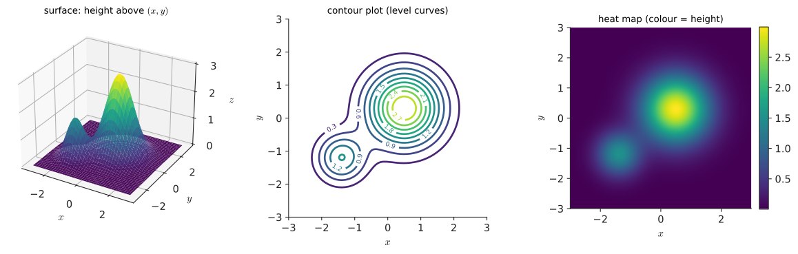
Contour plots are often more useful than surfaces. A surface hides its back side and is hard to read numerically. A contour plot shows everything at once, and the spacing of the contours tells you about steepness: closely packed contours mean steep ground, widely spaced contours mean gentle ground. Hold on to that sentence. It comes back when we meet the gradient.
20.1.3. Vocabulary and notation
|
Function of several variables
A function of several variables (or multivariable function) takes more than one input number and returns one output number. For example, \(f(x, y) = x^2 + 3y^2\) takes two inputs, and \(T(x, y, z)\) could give the temperature at a point in a room. A scalar-valued function returns a single number. (A function returning several numbers, such as a position in space, is vector-valued. We’ll meet one when we discuss the Jacobian.) |
|
ℝ², ℝⁿ, and bold vectors
\(\mathbb{R}\) is the set of real numbers. \(\mathbb{R}^2\) is the set of all ordered pairs \((x, y)\) of real numbers, i.e. the plane. \(\mathbb{R}^n\) is the set of all ordered lists of \(n\) real numbers, \((x_1, x_2, \ldots, x_n)\). So \(f : \mathbb{R}^2 \to \mathbb{R}\) reads "\(f\) takes a pair of reals to a real". When there are many inputs we bundle them into one object written in bold: \(\mathbf{x} = (x_1, x_2, \ldots, x_n)\), and write \(f(\mathbf{x})\) instead of \(f(x_1, \ldots, x_n)\). In handwriting, bold becomes an underline or an arrow: \(\vec{x}\). A model with a million weights is just a function \(L : \mathbb{R}^{1\,000\,000} \to \mathbb{R}\). |
|
Surface, level curve, contour
The graph (or surface) of \(f(x, y)\) is the set of points \((x, y, z)\) with \(z = f(x, y)\). A level curve of \(f\) at level \(c\) is the set of points in the plane where \(f(x, y) = c\). A contour plot draws several level curves at evenly spaced levels. With three inputs, the same idea gives level surfaces \(f(x, y, z) = c\). |
20.1.4. Worked example: level curves of a bowl
Take \(f(x, y) = x^2 + 3y^2\). What do its level curves look like? Try it: See the bowl’s elliptical level curves.
Set \(f(x, y) = c\) for a few values of \(c\):
Each level curve with \(c > 0\) is an ellipse. Along the \(x\)-axis, the \(c = 3\) ellipse reaches \(x = \pm\sqrt{3} \approx \pm 1.73\). Along the \(y\)-axis it reaches only \(y = \pm 1\). The ellipses are wider than they are tall, so the bowl rises more steeply in the \(y\) direction than in the \(x\) direction. That matches the formula: the coefficient 3 on \(y^2\) makes \(y\) count for more. Negative values of \(c\) give no level curve at all, because the bowl never goes below zero.
We’ll use this bowl later as the test case for gradient descent.
|
Contour spacing is not height
A contour plot shows height only through the labels on the curves. Two plots can look identical while describing hills of very different heights if their levels are spaced differently. Always check the contour interval. And remember that each curve is a set of points at one height. Moving along a contour does not change \(f\) at all. |
-
Everyday: body-mass index is a function of two variables, \(B(m, h) = m/h^2\) (mass in kg, height in m): 70 kg and 1.75 m give \(B = 70/1.75^2 \approx 22.9\). Weather maps (temperature and pressure over latitude and longitude), topographic maps, and the cost of a trip as a function of distance and fuel price are all functions of two or more inputs.
-
Science: the ideal gas law \(P = nRT/V\) makes pressure a function of temperature and volume. Potential energy over a region of space.
-
Computing: an image is a function \((\text{row}, \text{col}) \mapsto \text{brightness}\). The loss of a machine-learning model is a function of all of its parameters.
|
Explore a surface
Type a formula \(f(x, y)\) and see three linked views: the rotatable surface, the contour plot and the heat map. Hover over a point in any view to highlight it in the other two. Change the contour spacing and watch steep regions show up as bunched lines. Try it: Open the surface explorer |
20.2. Partial derivatives
20.2.1. The problem
On the hill \(h(x, y)\), "the slope" is ambiguous. The ground can climb steeply to the north and be level to the east at the same point. The derivative of Chapter 17 asked how the output changes when the single input changes. Now there are two inputs, so we have to ask a more specific question: how does the output change when one input changes and the others stay put?
20.2.2. Intuition: freeze everything else
Here is the key move, and it’s simpler than it sounds. Freeze all inputs but one. Then the function really is a function of one variable, and you already know how to differentiate it.
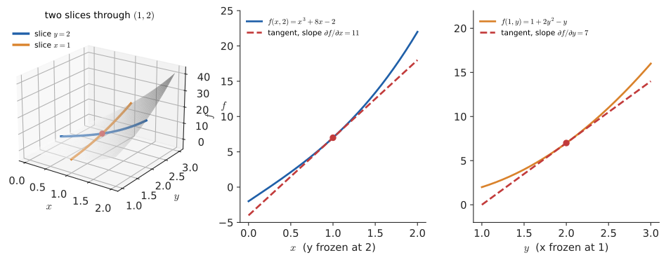
Geometrically, freezing \(y = 2\) slices the surface with the vertical plane \(y = 2\). The slice is an ordinary curve, and its slope at a point is the partial derivative with respect to \(x\). Freezing \(x\) instead slices in the other direction and gives the partial derivative with respect to \(y\).
20.2.3. Why it works: the definition
The partial derivative is the single-variable derivative applied to a slice, so its definition is the familiar limit with only one input nudged:
Look at what changes in each numerator. In the first, only the first argument moves (\(a \to a + h\)) and \(b\) is untouched. In the second, only \(b\) moves. Nothing else is new. Every rule from Chapter 17 (power, product, quotient, chain) still works. The one new habit is to treat the frozen variables as constants.
20.2.4. Vocabulary and notation
|
Partial derivative and the symbol ∂
The partial derivative of \(f\) with respect to \(x\) is the rate of change of \(f\) as \(x\) varies with every other input held fixed. Notations, all meaning the same thing:
\[\frac{\partial f}{\partial x}, \qquad f_x, \qquad \partial_x f, \qquad D_x f.\]
The curly \(\partial\) is read "partial" (or "del", or "dee"). It replaces the straight \(d\) of \(\frac{df}{dx}\) as a reminder that other variables exist and are being held fixed. To evaluate at a point, write \(\frac{\partial f}{\partial x}(1, 2)\) or \(f_x(1, 2)\). |
|
Second and mixed partial derivatives
Differentiating a partial derivative again gives a second partial derivative:
\[f_{xx} = \frac{\partial^2 f}{\partial x^2}, \qquad
f_{yy} = \frac{\partial^2 f}{\partial y^2}, \qquad
f_{xy} = \frac{\partial}{\partial y}\!\left(\frac{\partial f}{\partial x}\right) = \frac{\partial^2 f}{\partial y\,\partial x}.\]
\(f_{xy}\) and \(f_{yx}\) are mixed partials. For every function you will meet in practice (any function whose second partials are continuous), Clairaut’s theorem says they are equal: \(f_{xy} = f_{yx}\). The order of differentiation does not matter. |
20.2.5. The method
Input: a formula \(f(x_1, \ldots, x_n)\) and the variable \(x_i\) to differentiate with respect to.
Steps:
-
Mentally replace every variable except \(x_i\) by a constant. It can help to circle them or rename them \(a, b, \ldots\).
-
Differentiate with respect to \(x_i\) using the ordinary single-variable rules. A term with no \(x_i\) in it is a constant, so its derivative is 0. A constant factor multiplying \(x_i\) stays as a factor.
-
Restore the frozen variables. Substitute a point if one is given.
Output: the partial derivative \(\partial f / \partial x_i\), as a formula or as a number at a point.
20.2.6. Worked example
Find both partial derivatives of Try it: Partials as slices at (1, 2).
at the point \((1, 2)\).
With respect to \(x\) (freeze \(y\), so \(y^2\) behaves like a number such as 4):
With respect to \(y\) (freeze \(x\)):
At \((1, 2)\):
Interpretation. Standing at \((1, 2)\), where \(f(1,2) = 1 + 8 - 2 = 7\), a small step \(\Delta x\) east changes \(f\) by about \(11\,\Delta x\). A small step \(\Delta y\) north changes it by about \(7\,\Delta y\). These are the slopes of the two dashed tangent lines in the slice figure above.
Second partials (we’ll need them for the Hessian):
The mixed partials agree, as Clairaut promised. At \((1, 2)\): \(f_{xx} = 6\), \(f_{yy} = 4\), \(f_{xy} = 8\).
20.2.7. Alternative approach: numerical partial derivatives
When you have code for \(f\) but no formula, or you just want to check your algebra, approximate each partial with a central difference. Nudge one input up and down by a small \(h\) and leave the others alone:
def f(x, y):
    return x**3 + 2*x*y**2 - y

def partial_x(f, x, y, h=1e-6):
    return (f(x + h, y) - f(x - h, y)) / (2*h)   # y held fixed

def partial_y(f, x, y, h=1e-6):
    return (f(x, y + h) - f(x, y - h)) / (2*h)   # x held fixed

print(round(partial_x(f, 1, 2), 6), round(partial_y(f, 1, 2), 6))
11.0 7.0
Choosing a method. Use the symbolic rules whenever you have a formula. They give exact answers and formulas you can reuse. Use finite differences to check symbolic or hand-coded derivatives, or when \(f\) is a black box. Avoid them as the main tool when there are many inputs: each partial costs two function evaluations, so a function of a million variables would need two million evaluations per gradient. Chapter 32 explains why \(h\) can be neither too large nor too small.
|
What counts as a constant
The most common slip is differentiating a frozen variable anyway. With respect to \(x\):
A useful self-check: in \(\partial f/\partial x\), any term without an \(x\) must disappear. |
-
Health: for BMI \(B = m/h^2\), \(\partial B/\partial m = 1/h^2 \approx 0.33\) per kg and \(\partial B/\partial h = -2m/h^3 \approx -26\) per metre at 70 kg and 1.75 m. So gaining 1 kg raises BMI by about 0.33, while a height measurement that is 1 cm too short raises it by about 0.26. A careless tape measure matters almost as much as a kilogram.
-
Economics: the marginal product of labour is \(\partial Q / \partial L\) for a production function \(Q(L, K)\), meaning the extra output from one more worker with capital fixed. For the classic Cobb–Douglas form \(Q = 10L^{1/2}K^{1/2}\) with 100 workers and 400 units of capital, \(Q = 2000\) and \(\partial Q/\partial L = 5\sqrt{K/L} = 10\): one more worker adds about 10 units of output, while \(\partial Q/\partial K = 5\sqrt{L/K} = 2.5\) per unit of capital.
-
Physics: in thermodynamics, \((\partial P / \partial T)_V\) is how pressure rises with temperature at constant volume. The subscript \(V\) states explicitly what is held fixed.
-
Sensitivity analysis: in any model, \(\partial(\text{output}) / \partial(\text{parameter})\) measures how much one assumption matters while the others stay put.
|
Where did ∂ come from?
The curly \(\partial\) is a rounded letter d. Adrien-Marie Legendre used it in 1786 for partial derivatives, then abandoned it. Carl Jacobi revived it in 1841, and it has stuck ever since. Typesetters and programmers call it "del", "partial" or "curly d". In LaTeX it is |
20.2.8. Exercises
-
Find \(f_x\) and \(f_y\) for \(f(x, y) = 5x^2y^3\).
-
Find \(g_x\) and \(g_y\) for \(g(x, y) = e^{xy} + \ln y\).
-
Find all three first partial derivatives of \(h(x, y, z) = xyz + z^2\).
-
Verify that \(f_{xy} = f_{yx}\) for \(f(x, y) = x^2y^3\).
-
A rectangular box has volume \(V(l, w, h) = lwh\). Compute \(\partial V/\partial h\) at \((l, w, h) = (3, 2, 5)\) and explain what it means physically.
Answers
-
\(f_x = 10xy^3\) (\(5y^3\) is a constant factor; differentiate \(x^2\)). \(f_y = 15x^2y^2\) (\(5x^2\) is constant; differentiate \(y^3\)).
-
\(g_x = y\,e^{xy}\) (chain rule, inner derivative \(\partial(xy)/\partial x = y\); \(\ln y\) is constant). \(g_y = x\,e^{xy} + \frac{1}{y}\).
-
\(h_x = yz\), \(h_y = xz\), \(h_z = xy + 2z\).
-
\(f_x = 2xy^3\), so \(f_{xy} = \partial_y(2xy^3) = 6xy^2\). \(f_y = 3x^2y^2\), so \(f_{yx} = \partial_x(3x^2y^2) = 6xy^2\). They are equal.
-
\(\partial V/\partial h = lw = 3 \cdot 2 = 6\). Raising the height by a small amount \(\Delta h\) adds about \(6\,\Delta h\) to the volume: a slab with the base area \(6\) and thickness \(\Delta h\).
20.3. The gradient
20.3.1. The problem
A function of \(n\) variables has \(n\) partial derivatives. Each one describes the slope in one axis direction. Keeping track of them separately is clumsy. More importantly, the hiker doesn’t only want to walk due east or due north. We want one object that captures all the slope information at a point and can answer questions about any direction. That object is the gradient.
20.3.2. A short refresher on vectors
The full story of vectors is in Chapter 26. For this chapter you need only the following.
|
Vector, length, unit vector
A vector in \(\mathbb{R}^2\) is an ordered pair \(\mathbf{v} = (v_1, v_2)\), pictured as an arrow from the origin to the point \((v_1, v_2)\). It has a direction and a length. The same idea works with \(n\) components. Its length (or magnitude, or norm) is \(|\mathbf{v}| = \sqrt{v_1^2 + v_2^2}\) (Pythagoras; see Chapter 10). A unit vector has length 1 and is used purely to indicate a direction. Any nonzero vector can be turned into one by dividing by its length: \(\mathbf{u} = \mathbf{v}/|\mathbf{v}|\). For example, \((3, 4)\) has length 5, so \((0.6,\, 0.8)\) is the unit vector in that direction. |
|
Dot product
The dot product of two vectors multiplies matching components and adds the results:
\[\mathbf{a} \cdot \mathbf{b} = a_1 b_1 + a_2 b_2 \;(+ \cdots + a_n b_n).\]
It also has a geometric meaning, which Chapter 26 derives from the law of cosines:
\[\mathbf{a} \cdot \mathbf{b} = |\mathbf{a}|\,|\mathbf{b}|\cos\theta,\]
where \(\theta\) is the angle between the arrows. So the dot product is largest when the vectors point the same way (\(\cos 0 = 1\)), zero when they are perpendicular (\(\cos 90^\circ = 0\)), and most negative when they point opposite ways. |
20.3.3. Definition
|
Gradient and the symbol ∇
The gradient of \(f(x_1, \ldots, x_n)\) is the vector of its partial derivatives:
\[\nabla f = \left( \frac{\partial f}{\partial x_1},\; \frac{\partial f}{\partial x_2},\; \ldots,\; \frac{\partial f}{\partial x_n} \right).\]
The symbol \(\nabla\) is called nabla (or "del"). Read \(\nabla f(\mathbf{x})\) as "the gradient of \(f\) at the point \(\mathbf{x}\)". It is a vector with one component for each input, and it can be different at every point. In some texts it is also written \(\operatorname{grad} f\) or \(\frac{\partial f}{\partial \mathbf{x}}\). |
For our running example \(f(x, y) = x^3 + 2xy^2 - y\), we already have both partials:
So far this is just packaging. The payoff is two geometric facts, which the next two sections prove:
-
Direction: \(\nabla f\) points in the direction in which \(f\) increases fastest.
-
Magnitude: \(|\nabla f|\) is that fastest rate of increase.
There is also a corollary: \(\nabla f\) is perpendicular to the contour line through the point.
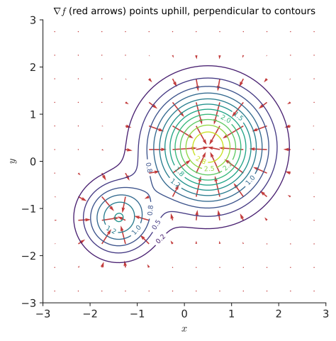
The arrows shrink to nothing at the two peaks. At a summit there is no uphill direction, so the gradient is the zero vector. Remember that observation: finding where \(\nabla f = \mathbf{0}\) is how we will find maxima and minima. Try it: Explore the gradient field.
20.3.4. Where you’d use this
-
Everyday: skiing and water. On a hillside, the direction of \(-\nabla h\) is the fall line: the way a ball rolls, water drains and a skier picks up speed fastest. Drainage engineers and hydrologists compute it from digital elevation maps to predict where floodwater will collect.
-
Physics and engineering: heat flow. Heat flows down the temperature gradient: Fourier’s law says the heat flux is \(-k\nabla T\). If the temperature falls by 20 °C across a 10 cm brick wall, \(|\nabla T| = 20/0.1 = 200\) °C per metre, and with brick’s conductivity \(k \approx 0.7\) W/(m·K) about 140 watts leak through every square metre. The same law with different letters governs diffusion of chemicals and the flow of groundwater; and in mechanics, force is minus the gradient of potential energy, \(\mathbf{F} = -\nabla U\).
-
Computing: edge detection. Treat a greyscale image as a function \(I(x, y)\). Where brightness jumps from 50 to 200 across a boundary, the central-difference gradient is about \((200 - 50)/2 = 75\) per pixel pointing across the boundary, and nearly zero along it. Edge detectors (Sobel, Canny) compute \(\nabla I\) at every pixel and mark points where \(|\nabla I|\) is large: the first stage of many computer-vision pipelines, from barcode scanners to lane detection in cars.
20.4. Tangent planes and linearisation
20.4.1. The problem
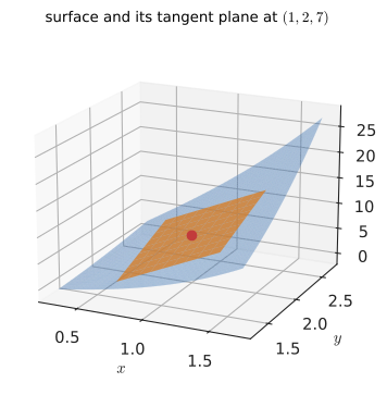
In one variable, the tangent line \(y = f(a) + f'(a)(x - a)\) was the best straight-line approximation to a curve near \(a\). Close to \(a\), the curve and the line are almost the same. What is the multivariable version? Zoom in far enough on a smooth surface and it looks flat, like the ground under your feet on a round Earth. That flat thing is the tangent plane.
20.4.2. Why it works
Move from \((a, b)\) to \((a + \Delta x,\, b + \Delta y)\). Do it in two legs: first east, then north.
-
The east leg changes \(f\) by about \(f_x(a, b)\,\Delta x\), since \(f_x\) is the slope in that direction.
-
The north leg changes \(f\) by about \(f_y\,\Delta y\). (Strictly, \(f_y\) is evaluated at the end of the first leg, but for small steps that is almost the same point.)
The two changes add:
Written with \(x = a + \Delta x\) and \(y = b + \Delta y\), this is the tangent plane at \((a, b)\):
In vector form, using the gradient and the dot product, it reads almost exactly like the one-variable tangent line:
This is the most important formula in the chapter. The gradient is the thing you dot with a small step to get the change in \(f\). It works unchanged in a million dimensions.
|
Linearisation, tangent plane, differential
The linearisation (or linear approximation) of \(f\) at \(\mathbf{a}\) is \(L(\mathbf{x}) = f(\mathbf{a}) + \nabla f(\mathbf{a}) \cdot (\mathbf{x} - \mathbf{a})\). Its graph, for two inputs, is the tangent plane. The total differential writes the same idea in terms of small changes: \(df = f_x\,dx + f_y\,dy\). |
20.4.3. Worked example
Find the tangent plane to \(f(x, y) = x^3 + 2xy^2 - y\) at \((1, 2)\), and use it to estimate \(f(1.1,\, 1.9)\). Try it: Tangent plane and its error.
The true value is \(f(1.1, 1.9) = 1.331 + 2(1.1)(3.61) - 1.9 = 1.331 + 7.942 - 1.9 = 7.373\). The estimate is off by 0.027, under 0.4%, for a step of 0.1 in each direction.
20.4.4. Application: propagating measurement error
You measure a rectangle as \(x = 20\) cm by \(y = 10\) cm, and each measurement may be off by up to \(0.1\) cm. How uncertain is the area \(A = xy\)? Try it: Propagate the measurement error.
So \(A = 200 \pm 3\) cm², about 1.5%. Notice that the error in the short side matters more, because it gets multiplied by the long side. Engineers and experimental scientists use this calculation every day under the name propagation of uncertainty.
20.5. Directional derivatives and the direction of steepest ascent
20.5.1. The problem
Our hiker at \((1, 2)\) on \(f(x, y) = x^3 + 2xy^2 - y\) wants to walk in the direction of the unit vector \(\mathbf{u} = (0.6,\, 0.8)\), roughly north-north-east. How fast does height change per unit distance walked? And of all possible directions, which climbs fastest?
20.5.2. Why it works: derive the directional derivative
Take a small step of length \(h\) in direction \(\mathbf{u}\), so \(\Delta\mathbf{x} = h\mathbf{u}\). Linearisation says:
As \(h \to 0\) the approximation becomes exact (for smooth \(f\)), which gives the directional derivative:
The partial derivatives are special cases. With \(\mathbf{u} = (1, 0)\) (due east), \(D_{\mathbf{u}} f = f_x\). With \(\mathbf{u} = (0, 1)\), \(D_{\mathbf{u}} f = f_y\).
|
Directional derivative
The directional derivative \(D_{\mathbf{u}} f(\mathbf{a})\) is the rate of change of \(f\) at \(\mathbf{a}\) per unit distance moved in the direction of the unit vector \(\mathbf{u}\). It equals \(\nabla f(\mathbf{a}) \cdot \mathbf{u}\). |
20.5.3. Why the gradient is the steepest direction
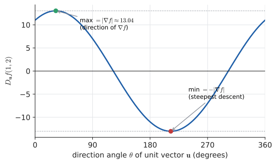
Now use the geometric form of the dot product. Let \(\theta\) be the angle between \(\nabla f\) and \(\mathbf{u}\). Since \(|\mathbf{u}| = 1\):
Read off the consequences. \(|\nabla f|\) is fixed at the point, so only \(\cos\theta\) varies as you turn to face different directions.
-
\(\cos\theta\) is largest, equal to 1, when \(\theta = 0\): when you face along \(\nabla f\). The rate of climb is then \(|\nabla f|\). The gradient points in the direction of steepest ascent, and its length is the steepest slope.
-
\(\cos\theta = -1\) when \(\theta = 180^\circ\): facing along \(-\nabla f\) gives the steepest descent, at rate \(-|\nabla f|\). That is the direction gradient descent will use.
-
\(\cos\theta = 0\) when \(\theta = 90^\circ\): walking perpendicular to the gradient, height doesn’t change at all, to first order. But a path along which height doesn’t change is exactly a contour line. So the gradient is perpendicular to the contour through the point.
That is the whole argument, and it rests on one fact about the dot product. It also explains the contour rule from the start of the chapter: bunched contours mean the height changes a lot over a short distance, so \(|\nabla f|\) is large.
20.5.4. The method
Input: a differentiable \(f\), a point \(\mathbf{a}\), and a direction vector \(\mathbf{v}\) (any length).
Steps:
-
Compute the gradient \(\nabla f(\mathbf{a})\) from the partial derivatives.
-
Normalise the direction: \(\mathbf{u} = \mathbf{v}/|\mathbf{v}|\).
-
Directional derivative: \(D_{\mathbf{u}} f(\mathbf{a}) = \nabla f(\mathbf{a}) \cdot \mathbf{u}\).
-
Steepest ascent direction: \(\nabla f(\mathbf{a}) / |\nabla f(\mathbf{a})|\), with rate \(|\nabla f(\mathbf{a})|\).
-
Steepest descent direction: \(-\nabla f(\mathbf{a}) / |\nabla f(\mathbf{a})|\), with rate \(-|\nabla f(\mathbf{a})|\).
Output: the rate of change in the requested direction, and the best and worst directions.
20.5.5. Worked example
At \((1, 2)\) on \(f(x, y) = x^3 + 2xy^2 - y\), with direction \(\mathbf{v} = (3, 4)\): Try it: Turn the direction dial.
So walking north-north-east climbs at 12.2 units of height per unit of distance. That is close to the best possible 13.04, because \((0.6, 0.8)\) points at about 53° and the gradient at about 32.5°, only 20° apart: \(13.04 \cos 20.6^\circ \approx 12.2\). Walking in direction \((-0.844, -0.537)\) descends fastest. Walking in direction \((-7, 11)/\sqrt{170}\), perpendicular to the gradient, keeps you on the contour \(f = 7\).
|
The direction must be a unit vector
\(\nabla f \cdot \mathbf{v}\) with an unnormalised \(\mathbf{v}\) gives the wrong number. With \(\mathbf{v} = (3, 4)\) above, you’d get \(33 + 28 = 61\), five times too big, because \(|\mathbf{v}| = 5\). Normalise first. Also, "the gradient points uphill" is a local statement. It gives the steepest direction right here. It does not point at the summit. On a curved ridge, following the gradient traces a curving path, as the arrows in the gradient-field figure show. |
20.5.6. Reading \(\nabla f(\mathbf{x})\) fluently
This is the literacy goal from the preface. When you meet
in a paper, unpack it in four layers:
-
Symbols: \(f\) is a scalar function of many variables. The bold \(\mathbf{x}\) is the point (a vector of inputs) where we evaluate. \(\nabla\) means "the gradient of".
-
Definition: it is a vector of partial derivatives, \(\big(\partial f/\partial x_1, \ldots, \partial f/\partial x_n\big)\), with one entry per input. Entry \(i\) says how sensitive \(f\) is to input \(i\) alone.
-
Geometry: it points in the direction of steepest increase of \(f\), its length is that steepest rate, and it is perpendicular to the level set through \(\mathbf{x}\).
-
Use: an optimisation algorithm uses it to decide which way to move. Step along \(-\nabla f\) to decrease \(f\) (gradient descent) or along \(+\nabla f\) to increase it.
If you can say those four sentences without looking, you have the main idea of this chapter.
|
Why "nabla"?
\(\nabla\) is an upside-down Greek capital delta. The name "nabla" comes from the Greek for a Hebrew harp that has roughly that triangular shape. William Rowan Hamilton introduced the symbol (lying on its side) in the 1840s. The physicist Peter Guthrie Tait set it upright. The name was suggested to Tait by the biblical scholar William Robertson Smith, and James Clerk Maxwell used it, half in jest, in his letters. Physicists mostly call it "del". |
|
Follow the arrow
Click a point on a contour map. The app draws \(\nabla f\) there and a draggable unit vector \(\mathbf{u}\). As you rotate \(\mathbf{u}\), a live readout shows \(D_{\mathbf{u}} f = |\nabla f|\cos\theta\) and a dot moves along the cosine wave. Confirm by hand that the maximum is along the gradient and the zeros are along the contour. Try it: Open the Follow the arrow lab |
20.5.7. Exercises
-
Compute \(\nabla f(3, 1)\) for \(f(x, y) = x^2 + 3y^2\), and give the unit vector in the direction of steepest descent there.
-
For \(f(x, y) = x^2 y\) at \((2, 1)\), find the directional derivative towards the point \((5, 5)\), and the maximum rate of increase.
-
For \(f(x, y) = x^2 + y^2\), verify that \(\nabla f(3, 4)\) is perpendicular to the level curve through \((3, 4)\). (Hint: the level curve is a circle. Its tangent direction at \((3,4)\) is \((-4, 3)\).)
-
Use linearisation to estimate \(\sqrt{3.1^2 + 3.9^2}\) from the point \((3, 4)\), and compare with the true value.
Answers
-
\(\nabla f = (2x, 6y)\), so \(\nabla f(3, 1) = (6, 6)\), with length \(\sqrt{72} = 6\sqrt{2}\). Steepest descent: \(-(6, 6)/(6\sqrt 2) = (-1/\sqrt 2, -1/\sqrt 2) \approx (-0.707, -0.707)\).
-
\(\nabla f = (2xy, x^2) = (4, 4)\) at \((2, 1)\). Direction \((5, 5) - (2, 1) = (3, 4)\), so \(\mathbf{u} = (0.6, 0.8)\). \(D_{\mathbf{u}} f = 4(0.6) + 4(0.8) = 2.4 + 3.2 = 5.6\). Maximum rate \(|\nabla f| = 4\sqrt 2 \approx 5.657\).
-
\(\nabla f = (2x, 2y) = (6, 8)\). Dot with the tangent direction: \((6)(-4) + (8)(3) = -24 + 24 = 0\), so they are perpendicular. The gradient points radially outwards, straight away from the circle’s centre.
-
\(f = \sqrt{x^2 + y^2}\), \(f(3, 4) = 5\), \(f_x = x/f = 0.6\), \(f_y = y/f = 0.8\). \(L = 5 + 0.6(0.1) + 0.8(-0.1) = 5 + 0.06 - 0.08 = 4.98\). True value: \(\sqrt{9.61 + 15.21} = \sqrt{24.82} \approx 4.98197\).
20.6. The multivariable chain rule
20.6.1. The problem
A drone flies a path \((x(t), y(t))\) through a room where the temperature is \(T(x, y)\). Its sensor reads \(T(x(t), y(t))\), a function of time alone. How fast does the reading change? It changes for two reasons: \(x\) is changing, and \(y\) is changing. We need a way to combine them.
20.6.2. Intuition and derivation
Over a short time \(\Delta t\), the drone moves by \(\Delta x \approx x'(t)\,\Delta t\) and \(\Delta y \approx y'(t)\,\Delta t\). Linearisation says the temperature changes by
Divide by \(\Delta t\) and let \(\Delta t \to 0\):
where \(\mathbf{r}'(t) = (x'(t), y'(t))\) is the drone’s velocity. The single-variable chain rule "multiply the rates" becomes "multiply along each path of dependence, then add over the paths". A tree diagram makes the bookkeeping mechanical.
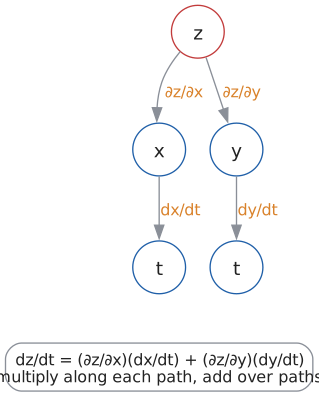
The same rule handles intermediate variables that depend on several inputs. If \(z = f(x, y)\) with \(x = x(s, t)\) and \(y = y(s, t)\), then
Input: an outer function \(z = f(x_1, \ldots, x_n)\) whose inputs depend on further variables. The goal is the derivative of \(z\) with respect to one of those further variables, \(t\).
Steps:
-
Draw the dependency tree from \(z\) down to every occurrence of \(t\).
-
Label each edge with the corresponding (partial) derivative.
-
For each path from \(z\) to \(t\), multiply the edge labels.
-
Add the products over all paths.
-
Substitute the current values of all variables.
Output: \(\partial z / \partial t\) (or \(dz/dt\) if \(t\) is the only underlying variable).
20.6.3. Worked example
The temperature is \(T(x, y) = x^2 + xy\) and the drone flies around the unit circle, \(x = \cos t\), \(y = \sin t\). Find \(dT/dt\) at \(t = \pi/4\).
At \(t = \pi/4\), \(x = y = \sin(\pi/4) = \cos(\pi/4) = \tfrac{\sqrt2}{2}\):
Check by the alternative method. Substitute first and use one-variable calculus. \(T(t) = \cos^2 t + \cos t \sin t = \cos^2 t + \tfrac12\sin 2t\). Then \(T'(t) = -2\cos t\sin t + \cos 2t = -\sin 2t + \cos 2t\), and \(T'(\pi/4) = -1 + 0 = -1\). The answers agree.
Choosing a method. For a small problem with explicit formulas, substituting first is often quicker. The chain-rule form wins when the functions are only known numerically, when there are many intermediate variables, or when you need the derivatives with respect to many inputs at once. That last case is what neural networks require.
Where you’d use this. Any sensor moving through a field measures a chain-rule derivative. A drone flying at velocity \((5, 3)\) m/s through air where \(\nabla T = (-0.02, 0.01)\) °C per metre sees its temperature reading change at \(\frac{dT}{dt} = T_x\frac{dx}{dt} + T_y\frac{dy}{dt} = (-0.02)(5) + (0.01)(3) = -0.07\) °C per second, about 4 °C a minute, even if the air itself is not changing at all. Weather balloons, ocean gliders and a phone’s barometric altimeter all rely on this split between "the field changed" and "I moved through the field". In economics, the same formula says how a cost index moves when several prices drift at once.
20.6.4. The Jacobian, briefly
So far the outer function returned a single number. Many maps return several numbers: a robot arm maps joint angles \((\theta_1, \theta_2)\) to a hand position \((x, y)\). A graphics transform maps \((u, v)\) texture coordinates to screen positions. For a map \(\mathbf{F} : \mathbb{R}^n \to \mathbb{R}^m\), put the gradients of the \(m\) output components in the rows of a matrix:
|
Jacobian matrix
The Jacobian of \(\mathbf{F}(x, y) = \big(F_1(x, y), F_2(x, y)\big)\) is the matrix of all first partial derivatives:
\[J = \begin{bmatrix} \dfrac{\partial F_1}{\partial x} & \dfrac{\partial F_1}{\partial y} \\[2mm] \dfrac{\partial F_2}{\partial x} & \dfrac{\partial F_2}{\partial y} \end{bmatrix}.\]
Row \(i\) is \(\nabla F_i\). The Jacobian is the multi-output version of the derivative: small input changes \(\Delta\mathbf{x}\) produce output changes \(\Delta\mathbf{F} \approx J\,\Delta\mathbf{x}\). Matrix–vector multiplication is explained in Chapter 27. |
Example: the polar-to-Cartesian map \(x = r\cos\theta,\ y = r\sin\theta\) has Jacobian
The determinant \(r\) is the area-scaling factor. That’s why a small polar rectangle has area \(r\,dr\,d\theta\), a fact we’ll use for double integrals. In robotics, the Jacobian of the arm’s kinematics converts joint speeds into hand velocity. Inverting it ("which joint speeds give the hand velocity I want?") is the core of real-time arm control. The arm is in trouble exactly where \(\det J = 0\), a singular configuration such as a fully outstretched arm, which cannot move its hand any further outward.
|
Leibniz’s notation pays off
The chain rule \(\frac{dz}{dt} = \frac{\partial z}{\partial x}\frac{dx}{dt} + \cdots\) looks as if the \(\partial x\) and \(dx\) "cancel". They don’t really, because a partial derivative is not a fraction, and in some thermodynamics identities naive cancellation gives the wrong sign. Still, the notation was designed to suggest the right answer most of the time, and it is one reason Leibniz’s notation beat Newton’s dots. |
20.6.5. Exercises
-
Let \(z = x^2y\) with \(x = t^2\) and \(y = 3t\). Find \(dz/dt\) at \(t = 1\) by the chain rule, then check by substituting first.
-
Draw the dependency tree for \(w = f(x, y, z)\) with \(x, y, z\) each a function of \(s\) and \(t\), and write the formula for \(\partial w / \partial s\).
-
In the neuron example, compute \(\partial L/\partial w\) when \(x = 1\), \(y = 0\), \(w = 2\), \(b = 1\). Which way should \(w\) move to reduce the loss?
Answers
-
\(z_x = 2xy\), \(z_y = x^2\), \(x' = 2t\), \(y' = 3\). At \(t = 1\): \(x = 1, y = 3\). \(dz/dt = (2 \cdot 1 \cdot 3)(2) + (1)(3) = 12 + 3 = 15\). Check: \(z = t^4 \cdot 3t = 3t^5\), so \(dz/dt = 15t^4 = 15\) at \(t = 1\).
-
Three paths from \(w\) to \(s\): \(\frac{\partial w}{\partial s} = \frac{\partial w}{\partial x}\frac{\partial x}{\partial s} + \frac{\partial w}{\partial y}\frac{\partial y}{\partial s} + \frac{\partial w}{\partial z}\frac{\partial z}{\partial s}\).
-
\(p = 2(1) + 1 = 3\), \(\partial L/\partial p = 2(3 - 0) = 6\), \(\partial L/\partial w = 6 \cdot x = 6\). The derivative is positive, so decrease \(w\) to reduce the loss.
20.7. Critical points and the Hessian
20.7.1. The problem
In Chapter 18 you found the maxima and minima of \(f(x)\) by solving \(f'(x) = 0\) and then checking the second derivative. What is the multivariable version, and what new possibilities appear when there is more than one direction?
20.7.2. Intuition
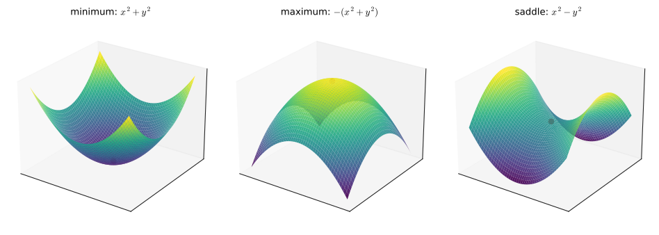
At the top of a smooth hill or the bottom of a smooth bowl, the ground is level in every direction: the tangent plane is horizontal. That means every directional derivative is zero, which happens exactly when \(\nabla f = \mathbf{0}\).
But a level tangent plane does not guarantee a peak or a pit. Think of a horse saddle or a mountain pass. Along the path over the pass you are at a high point. Along the ridge that the pass cuts through you are at a low point. The tangent plane is horizontal, yet the point is neither a maximum nor a minimum. This saddle point has no counterpart worth mentioning in one variable, and it turns out to be extremely common in high dimensions.
|
Critical point, saddle point, Hessian
A critical point (or stationary point) of \(f\) is a point where \(\nabla f = \mathbf{0}\), i.e. every first partial derivative is zero. A saddle point is a critical point that is neither a local maximum nor a local minimum: \(f\) rises in some directions and falls in others. The Hessian is the matrix of second partial derivatives:
\[H = \begin{bmatrix} f_{xx} & f_{xy} \\ f_{yx} & f_{yy} \end{bmatrix}.\]
It is symmetric (\(f_{xy} = f_{yx}\)) and plays the role of the second derivative: it measures curvature. |
20.7.3. Why it works: the second-derivative test
Near a critical point the linear term of the approximation vanishes (the gradient is zero), so the shape is decided by the next term, the quadratic one built from the Hessian. For two variables, the type of that quadratic is decided by one number, the discriminant
Roughly: if \(D > 0\), the surface curves the same way in every direction (a bowl or a dome), and the sign of \(f_{xx}\) says which. If \(D < 0\), it curves up in some directions and down in others, which is a saddle. For the general \(n\)-variable picture, the signs of the Hessian’s eigenvalues decide: all positive means a minimum, all negative a maximum, mixed a saddle. That’s one of the reasons Chapter 28 matters.
Input: a function \(f(x, y)\) with continuous second partials.
Steps:
-
Compute \(f_x\) and \(f_y\). Solve \(f_x = 0\) and \(f_y = 0\) simultaneously to get the critical points.
-
Compute \(f_{xx}\), \(f_{yy}\), \(f_{xy}\).
-
At each critical point evaluate \(D = f_{xx}f_{yy} - f_{xy}^2\).
-
\(D > 0\) and \(f_{xx} > 0\): local minimum. \(D > 0\) and \(f_{xx} < 0\): local maximum. \(D < 0\): saddle point. \(D = 0\): the test is inconclusive.
Output: each critical point with its classification.
20.7.4. Worked example
Classify the critical points of \(f(x, y) = x^3 - 3x + y^2\). Try it: Classify these critical points.
The local minimum value is \(f(1, 0) = 1 - 3 + 0 = -2\). Is it the global minimum? No. Along the \(x\)-axis, \(f(x, 0) = x^3 - 3x \to -\infty\) as \(x \to -\infty\), so the function has no lowest value at all. The second-derivative test is purely local.
|
Local is not global, and D = 0 tells you nothing
|
Try it: See D = 0 fail.
20.7.5. Where you’d use this
-
Science: fitting a line to data. "Least squares" chooses the slope \(m\) and intercept \(c\) that minimise \(S(m, c) = \sum_i (y_i - mx_i - c)^2\). Setting \(\nabla S = \mathbf{0}\) gives two linear equations (the normal equations). For the points \((1, 2)\), \((2, 3)\), \((3, 5)\) they give \(m = 1.5\), \(c = \tfrac13\), and the Hessian test (\(S_{mm} = 28\), \(S_{cc} = 6\), \(S_{mc} = 12\), \(D = 24 > 0\)) confirms a minimum. Every spreadsheet trendline and every linear-regression library starts here (Chapter 31).
-
Chemistry. A molecule’s energy is a function of all its atoms' positions. Stable molecules sit at minima; the transition state of a reaction, the highest point on the easiest path between reactant and product, is a saddle point, and chemistry software locates it with exactly the Hessian test above.
-
Computing. Machine-learning losses are classified the same way, as the sidebar below explains: the gradient finds the critical points, the Hessian says what kind they are.
|
Saddles dominate high dimensions
For a critical point to be a minimum in \(n\) dimensions, the surface must curve upward in every one of \(n\) independent directions. If each direction were a coin flip, the chance would be \(2^{-n}\). In a million dimensions, almost every critical point is a saddle. Research in the 2010s suggested that this, rather than "bad local minima", is the main geometric obstacle in training deep networks, and that noisy gradient methods are good at slipping off saddles. |
20.8. Gradient descent
20.8.1. The problem
You want the minimum of a function \(f(\mathbf{x})\): the loss of a model, the energy of a molecule, the cost of a design. You can compute \(f\) and \(\nabla f\) at any point, but solving \(\nabla f = \mathbf{0}\) symbolically is impossible, because there are too many variables and the equations are too tangled. What can you do?
20.8.2. Intuition: walking downhill in fog
You are on a mountainside in thick fog and want to reach the valley floor. You can’t see the valley, but you can feel the slope under your feet. A sensible strategy: feel which way is steepest downhill, take a step that way, and repeat. The gradient gives you exactly that local information. Steepest descent is the direction \(-\nabla f\), and that gives the iteration
Here \(\mathbf{x}_k\) is the position after \(k\) steps and \(\eta\) (Greek "eta") is the step-size multiplier.
20.8.3. Why it works
Linearisation tells us how much one step changes \(f\). With \(\Delta\mathbf{x} = -\eta\nabla f\):
Since \(|\nabla f|^2 > 0\) whenever we’re not at a critical point, a small enough positive \(\eta\) is guaranteed to decrease \(f\). The words "small enough" are where all the practical difficulty lives, because the linear approximation is only trustworthy for small steps. Notice also that the step length is \(\eta|\nabla f|\): steps are automatically long on steep ground and short on gentle ground, so the method slows down as it nears a minimum.
|
Learning rate, iterate, convergence
The learning rate (or step size) \(\eta\) is the positive number multiplying the gradient in each update. Machine learning calls it the learning rate. Numerical analysis calls it the step size and often writes \(\alpha\). Each \(\mathbf{x}_k\) is an iterate. The method converges if the iterates approach a limit (ideally a minimum), and diverges if they run off, typically growing without bound. |
20.8.4. The method
Input: a differentiable function \(f\) and a way to compute \(\nabla f\); a starting point \(\mathbf{x}_0\); a learning rate \(\eta > 0\); a tolerance \(\varepsilon\); an iteration cap \(K\).
Steps:
-
Set \(k = 0\).
-
Compute \(\mathbf{g} = \nabla f(\mathbf{x}_k)\).
-
If \(|\mathbf{g}| < \varepsilon\), stop: you are (nearly) at a critical point.
-
Update \(\mathbf{x}_{k+1} = \mathbf{x}_k - \eta\,\mathbf{g}\).
-
If the iterates are blowing up, or \(f\) is rising, stop and reduce \(\eta\).
-
Increase \(k\). If \(k < K\), go to step 2.
Output: \(\mathbf{x}_k\), an approximate local minimiser, and the number of steps taken.
20.8.5. Worked example: three steps by hand
Minimise \(f(x, y) = x^2 + 3y^2\) (the elliptical bowl from the first section) starting at \(\mathbf{x}_0 = (3, 1)\) with \(\eta = 0.1\). The gradient is \(\nabla f = (2x,\ 6y)\). Try it: Step down the bowl.
The loss falls 12 → 6.24 → 3.76 → 2.37. Look at the pattern in the coordinates. Each step multiplies \(x\) by 0.8 and \(y\) by 0.4. That’s no accident:
With \(\eta = 0.1\) the factors are \(0.8\) and \(0.4\). The \(y\) coordinate, in the steep direction, collapses quickly, while \(x\), in the shallow direction, shrinks only by 20% per step. That slow direction sets the overall pace.
20.8.6. Implementation and experiment
def gradient_descent(grad, x0, eta, tol=1e-8, max_iter=10_000):
    x = list(x0)
    for k in range(max_iter):
        g = grad(x)
        if sum(gi*gi for gi in g) ** 0.5 < tol:   # gradient ~ 0: stop
            return x, k
        x = [xi - eta*gi for xi, gi in zip(x, g)]  # step downhill
        if any(abs(xi) > 1e12 for xi in x):
            raise OverflowError(f"diverged at iteration {k}")
    return x, max_iter

grad = lambda p: [2*p[0], 6*p[1]]      # gradient of f(x, y) = x^2 + 3y^2

for eta in [0.01, 0.1, 0.25, 0.3, 0.34, 0.5]:
    try:
        x, k = gradient_descent(grad, [3.0, 1.0], eta)
        print(f"eta={eta:<5} converged in {k:5d} steps to "
              f"({x[0]:.1e}, {x[1]:.1e})")
    except OverflowError as e:
        print(f"eta={eta:<5} {e}")
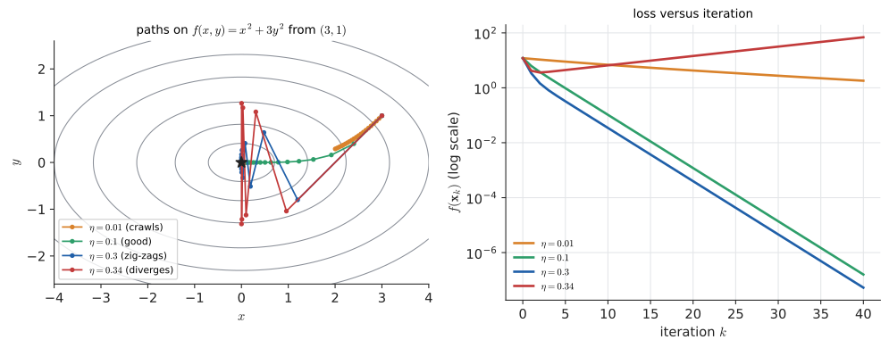
eta=0.01 converged in 1001 steps to (4.9e-09, 1.3e-27) eta=0.1 converged in 91 steps to (4.6e-09, 6.1e-37) eta=0.25 converged in 30 steps to (2.8e-09, 9.3e-10) eta=0.3 converged in 91 steps to (1.8e-36, -1.5e-09) eta=0.34 diverged at iteration 704 eta=0.5 diverged at iteration 39
The multiplier formulas explain every line of this output.
-
Too small (\(\eta = 0.01\)): the factors are 0.98 and 0.94. Every step is safe, but \(x\) shrinks by only 2% per step, so it takes over a thousand steps. The method crawls.
-
Good (\(\eta = 0.1\)): factors 0.8 and 0.4. Steady progress.
-
Best (\(\eta = 0.25\)): factors \(0.5\) and \(-0.5\). Both coordinates shrink at the same rate (the \(y\) coordinate flips sign each step but halves in size). This balances the slow and fast directions, and it is the fastest constant step for this bowl.
-
Getting large (\(\eta = 0.3\)): factors 0.4 and \(-0.8\). Now \(y\) is the slow coordinate, and it flips sign every step. The path zig-zags across the valley.
-
Too large (\(\eta = 0.34\)): the \(y\) factor is \(1 - 6(0.34) = -1.04\). Its magnitude exceeds 1, so \(y\) grows by 4% each step while bouncing side to side, and the iteration slowly diverges. At \(\eta = 0.5\) the factor is \(-2\) and the blow-up is fast.
So convergence requires \(|1 - 2\eta| < 1\) and \(|1 - 6\eta| < 1\), i.e. \(0 < \eta < 1/3\). The steepest direction sets the upper limit on the learning rate, and the shallowest direction sets the speed. The 2 and 6 are the eigenvalues of this bowl’s Hessian, \(H = \begin{bmatrix} 2 & 0 \\ 0 & 6 \end{bmatrix}\), and their ratio, the condition number \(6/2 = 3\), measures how elongated the bowl is. Long thin valleys (large condition number) are slow for gradient descent no matter how you tune \(\eta\). Chapter 28 and Chapter 32 develop that idea.
20.8.7. Alternative approaches and choosing a method
-
Solve \(\nabla f = \mathbf{0}\) exactly. Best when it’s possible: quadratic functions, a handful of variables, tidy formulas. Linear regression with squared loss can be solved this way via the "normal equations" (Chapter 33). Try it: Try learning rates yourself.
-
Newton’s method. Use the Hessian to build a quadratic model and jump to its minimum: \(\mathbf{x}_{k+1} = \mathbf{x}_k - H^{-1}\nabla f\). On our bowl it lands on the exact minimum in one step, because the bowl is quadratic. It converges very quickly near a minimum, but each step needs the \(n \times n\) Hessian and a linear solve, which is impossible for a million variables (a \(10^{12}\)-entry matrix).
-
Gradient descent and its relatives. Cheap per step (one gradient), scales to huge \(n\). The relatives (stochastic gradient descent, momentum, Adam) dominate machine learning and appear in Chapter 33.
-
Derivative-free methods (grid search, Nelder–Mead, evolutionary algorithms). Use these when no gradient is available or \(f\) is noisy or discontinuous. They are much slower in many dimensions.
Rule of thumb: few variables and a formula, solve analytically. Tens to thousands of smooth variables, use Newton-type or quasi-Newton methods (BFGS) from a library. Millions of variables, or data arriving in batches, use gradient descent variants.
|
How gradient descent fails
|
|
Cauchy, 1847
Gradient descent was proposed by Augustin-Louis Cauchy in 1847, in a short note on solving the systems of equations that arose in computing planetary orbits. He suggested reducing a positive function by stepping against its partial derivatives. A method designed to save astronomers some arithmetic now trains nearly every machine-learning model in the world. |
|
Tune the learning rate
Pick a surface (round bowl, elongated bowl, a banana-shaped Rosenbrock valley, a two-minimum landscape). Click to choose a starting point and drag a slider for \(\eta\). The app animates the descent path on the contour plot and draws the loss curve beside it. Find the largest \(\eta\) that still converges on the elongated bowl, and check it against the prediction \(2/\lambda_{\max}\). On the two-minimum landscape, colour each starting point by which minimum it reaches. |
20.8.8. Exercises
-
Do two steps of gradient descent by hand on \(f(x, y) = (x - 1)^2 + 2(y + 2)^2\) from \((0, 0)\) with \(\eta = 0.1\).
-
For the same function, what is the largest constant learning rate for which gradient descent converges from any start?
-
Explain in a sentence why the loss curve in the right-hand figure is a straight line on a log scale for \(\eta = 0.1\).
-
A colleague’s training loss goes 2.3, 2.1, 2.6, 4.9, 31, NaN. What is the most likely cause, and what should they try?
Answers
-
\(\nabla f = (2(x - 1),\ 4(y + 2))\). At \((0, 0)\): \((-2, 8)\), so \(\mathbf{x}_1 = (0 + 0.2,\ 0 - 0.8) = (0.2, -0.8)\). At \((0.2, -0.8)\): \(\nabla f = (-1.6,\ 4.8)\), so \(\mathbf{x}_2 = (0.2 + 0.16,\ -0.8 - 0.48) = (0.36, -1.28)\). Both coordinates head towards the minimum \((1, -2)\).
-
The error factors are \(1 - 2\eta\) for \(x\) and \(1 - 4\eta\) for \(y\). We need \(|1 - 4\eta| < 1\), so \(\eta < 0.5\). (The Hessian is \(\operatorname{diag}(2, 4)\) and \(2/\lambda_{\max} = 0.5\).)
-
Each step multiplies each coordinate by a fixed factor (0.8 or 0.4), so the loss is multiplied by roughly a fixed factor per step. Geometric decay \(c\,r^k\) has \(\log(c\,r^k) = \log c + k\log r\), which is linear in \(k\).
-
The learning rate is too large: the loss first falls, then oscillates and blows up. Reduce \(\eta\) (try one tenth), and consider gradient clipping or a warm-up schedule.
20.9. Constrained optimisation: Lagrange multipliers
20.9.1. The problem
You have 8 metres of fencing to build a rectangular pen against a long wall. The wall forms one side, so the fencing covers one side of length \(x\) parallel to the wall and two sides of length \(y\). Maximise the area \(A = xy\) subject to \(x + 2y = 8\).
This is optimisation with a constraint. You can’t wander freely over the \((x, y)\) plane, only along the line \(x + 2y = 8\). Real problems are full of constraints: budgets, capacities, physical laws, probabilities that must sum to 1.
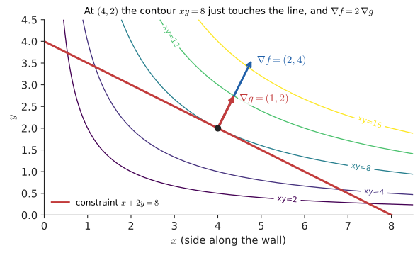
20.9.2. Intuition: the contour that just touches
Draw the contours of the objective \(f = xy\) and the constraint line. Walk along the line. As you go, you cross contours of higher and higher area, until you reach a point where the line only touches a contour without crossing it. Beyond it, you’d cross back to lower contours. At that touching point the constraint curve and the contour are tangent.
Two curves that are tangent at a point share a tangent line there, so their perpendiculars are parallel. The perpendicular to a contour of \(f\) is \(\nabla f\). The constraint curve is itself a contour of the function \(g(x, y) = x + 2y\), so its perpendicular is \(\nabla g\). Therefore, at the optimum,
|
Lagrange multiplier
To optimise \(f(\mathbf{x})\) subject to a constraint \(g(\mathbf{x}) = c\), look for points where \(\nabla f = \lambda\nabla g\) and \(g = c\). The number \(\lambda\) (Greek "lambda") is the Lagrange multiplier. It measures how fast the optimal value of \(f\) changes as the constraint level \(c\) is relaxed: \(\lambda = d f^*/dc\). Economists call it the shadow price of the constraint. |
Input: an objective \(f(x, y)\) and a constraint \(g(x, y) = c\).
Steps:
-
Compute \(\nabla f\) and \(\nabla g\).
-
Write the equations \(f_x = \lambda g_x\), \(f_y = \lambda g_y\), \(g(x, y) = c\): three equations in three unknowns \(x, y, \lambda\).
-
Solve them. It often helps to express \(x\) and \(y\) in terms of \(\lambda\), then substitute into the constraint.
-
Evaluate \(f\) at every solution (and at the ends of the constraint curve, if it has any). The largest value is the maximum, the smallest the minimum.
Output: the constrained optimum, its location, and \(\lambda\).
20.9.3. Worked example
Maximise \(f(x, y) = xy\) subject to \(g(x, y) = x + 2y = 8\). Try it: Watch the gradients align.
The ends of the feasible segment (\(x = 0\) or \(y = 0\)) give area 0, so \((4, 2)\) is the maximum. The side along the wall is twice each of the other sides.
Alternative: substitution. From the constraint, \(x = 8 - 2y\), so \(A(y) = (8 - 2y)y = 8y - 2y^2\). Then \(A'(y) = 8 - 4y = 0\) gives \(y = 2\), \(x = 4\). Same answer, with ordinary one-variable calculus.
Checking the meaning of \(\lambda\). With \(c\) metres of fence instead of 8, the same steps give \(\lambda = c/4\), \(x = c/2\), \(y = c/4\), so the best area is \(A^* = c^2/8\). Then \(dA^*/dc = c/4\), which equals 2 at \(c = 8\). That is exactly \(\lambda\). One extra metre of fence buys about 2 extra square metres of pen.
Choosing a method. Substitution is easier when you can solve the constraint for one variable cleanly. Lagrange multipliers win when you can’t (constraints like \(x^2 + xy + y^4 = 1\)), when there are many variables and constraints, when symmetry makes the \(\lambda\) equations easy, or when the value of \(\lambda\) itself is what you want to know.
|
Lagrange finds candidates, not answers
|
-
Economics: maximise utility subject to a budget. With £40 to spend on coffees at £2 and cakes at £4, and "utility" \(U = xy\), the condition \((y, x) = \lambda(2, 4)\) with \(2x + 4y = 40\) gives \(\lambda = 2.5\), so 10 coffees and 5 cakes. The multiplier is the marginal utility of money: one more pound of budget buys about 2.5 more units of utility. Try it: Coffee and cake, interactively.
-
Physics: a bead on a wire minimises energy subject to staying on the wire. \(\lambda\) turns out to be the constraint force.
-
Statistics and information theory: the maximum-entropy distribution with a given mean is found with Lagrange multipliers, and it is the exponential distribution (Chapter 30, Chapter 33).
-
Machine learning: support vector machines are formulated as constrained optimisation, and their famous "support vectors" are the data points whose multipliers are nonzero.
20.9.4. Exercises
-
Minimise \(x^2 + y^2\) subject to \(x + y = 4\), using Lagrange multipliers. Interpret geometrically.
-
Find the maximum and minimum of \(f(x, y) = x + y\) on the circle \(x^2 + y^2 = 2\). Try it: Check this exercise.
Answers
-
\(\nabla f = (2x, 2y) = \lambda(1, 1)\), so \(x = y = \lambda/2\). The constraint gives \(\lambda = 4\), so \(x = y = 2\) and the minimum is \(8\). Geometrically, \((2, 2)\) is the point of the line closest to the origin, at distance \(\sqrt 8 = 2\sqrt 2\). The smallest circle centred at the origin that touches the line touches it there.
-
\((1, 1) = \lambda(2x, 2y)\), so \(x = y = 1/(2\lambda)\). The constraint gives \(2/(4\lambda^2) = 2\), so \(\lambda = \pm\tfrac12\). \(\lambda = \tfrac12\) gives \((1, 1)\) with \(f = 2\) (maximum). \(\lambda = -\tfrac12\) gives \((-1, -1)\) with \(f = -2\) (minimum).
20.10. Double integrals
20.10.1. The problem
In Chapter 19, \(\int_a^b f(x)\,dx\) added up infinitely many thin strips to find the area under a curve. Now suppose \(f(x, y)\) is the depth of snow over a rectangular field. How much snow is there? You need the volume under the surface \(z = f(x, y)\) over a region of the plane.
20.10.2. Intuition and why it works
Chop the region into small rectangles of width \(\Delta x\) and depth \(\Delta y\). Over each one, stand a column whose height is the value of \(f\) at some sample point inside it. Each column has volume \(f \cdot \Delta x\,\Delta y\). Add them all up and refine the grid. The limit of these sums is the double integral:
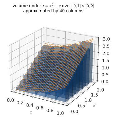
How do you compute it? Add the columns one row at a time. Fix \(x\) and integrate over \(y\). That gives the area of one vertical slice through the solid, a function of \(x\). Then integrate those slice areas over \(x\), exactly as you found volumes by slicing in Chapter 19. This is an iterated integral, and Fubini’s theorem guarantees that for continuous \(f\) on a rectangle, the order doesn’t matter:
|
Double integral, iterated integral, dA
The double integral \(\iint_R f\,dA\) is the signed volume between the surface \(z = f(x, y)\) and the region \(R\) of the plane. \(dA\) stands for a tiny element of area, \(dx\,dy\) in Cartesian coordinates and \(r\,dr\,d\theta\) in polar coordinates (the \(r\) is the Jacobian determinant from earlier). An iterated integral evaluates it as two ordinary integrals, inner first. While doing the inner integral, the outer variable is held constant, exactly as with partial derivatives. \(\lbrack a, b] \times [c, d]\) (read "\(a\) to \(b\) cross \(c\) to \(d\)") is the rectangle of points with \(a \le x \le b\) and \(c \le y \le d\). |
20.10.3. Worked example
Find \(\iint_R (x^2 + y)\,dA\) over \(R = [0, 1] \times [0, 2]\). Try it: Refine the columns.
Order 1: \(y\) inside. Hold \(x\) fixed:
Order 2: \(x\) inside. Hold \(y\) fixed:
Both orders give \(8/3 \approx 2.667\), as Fubini promised. Dividing by the area of \(R\) (which is 2) gives the average value of \(f\) over the region, \(4/3\).
20.10.4. Numerical check
The column picture translates directly into code, as the midpoint rule in two dimensions:
import numpy as np

def double_integral_midpoint(f, ax, bx, ay, by, n):
    dx, dy = (bx - ax)/n, (by - ay)/n
    xs = ax + dx*(np.arange(n) + 0.5)      # midpoints in x
    ys = ay + dy*(np.arange(n) + 0.5)      # midpoints in y
    X, Y = np.meshgrid(xs, ys)
    return f(X, Y).sum() * dx * dy        # sum of column volumes

f = lambda x, y: x**2 + y
for n in [5, 50, 500]:
    print(n, double_integral_midpoint(f, 0, 1, 0, 2, n))
print("exact", 8/3)
5 2.660000000000001 50 2.6666000000000003 500 2.666666 exact 2.6666666666666665
Each tenfold refinement cuts the error by a factor of 100, the \(O(h^2)\) behaviour of the midpoint rule. But in \(d\) dimensions an \(n\)-per-side grid needs \(n^d\) evaluations. That "curse of dimensionality" is why high-dimensional integrals (in physics, finance and Bayesian statistics) are done by Monte Carlo sampling instead, which Chapter 32 covers.
|
Non-rectangular regions
Over a region that isn’t a rectangle, the inner limits depend on the outer variable. Over the triangle \(0 \le y \le x \le 1\), for instance, you write \(\int_0^1 \int_0^x f\,dy\,dx\). Swapping the order means re-describing the region (\(\int_0^1 \int_y^1 f\,dx\,dy\)), not just swapping the symbols. Always sketch the region first. |
-
Probability: for two random variables with joint density \(p(x, y)\), probabilities are double integrals, \(P((X, Y) \in R) = \iint_R p\,dA\) (Chapter 30).
-
Physics: the mass of a plate with variable density, the centre of mass, the moment of inertia.
-
Environment: hydrologists find the total volume of rain falling on a catchment by integrating rainfall depth over its area. If the depth across a 3 km by 2 km catchment is \(r(x, y) = 10 + 2x\) mm (wetter towards the east), the total is \(\int_0^3\!\int_0^2 (10 + 2x)\,dy\,dx = 2(30 + 9) = 78\) mm·km², and since 1 mm over 1 km² is 1000 m³, that is 78,000 m³ of water heading for the river.
-
Graphics: rendering integrates incoming light over a hemisphere of directions at each pixel. Path tracers estimate those integrals by Monte Carlo.
20.10.5. Exercises
-
Evaluate \(\int_0^2\!\int_0^3 (2x + y)\,dy\,dx\) in both orders, and give the average value of \(2x + y\) over the rectangle.
-
Set up, but do not evaluate, the integral of \(f(x, y)\) over the triangle with vertices \((0, 0)\), \((2, 0)\), \((0, 2)\).
Answers
-
\(y\) inside: \(\int_0^3 (2x + y)\,dy = 6x + \tfrac92\), then \(\int_0^2 (6x + 4.5)\,dx = 12 + 9 = 21\). \(x\) inside: \(\int_0^2 (2x + y)\,dx = 4 + 2y\), then \(\int_0^3 (4 + 2y)\,dy = 12 + 9 = 21\). The area is 6, so the average value is \(21/6 = 3.5\).
-
The hypotenuse is \(x + y = 2\). With \(y\) inside: \(\int_0^2 \int_0^{2 - x} f(x, y)\,dy\,dx\).
20.11. Putting it together
Here is the chapter on one page, as a chain of ideas:
-
A function of several variables is a landscape. Picture it as a surface, contours or a heat map.
-
A partial derivative is the slope of a slice, with every other input frozen.
-
The gradient \(\nabla f\) bundles the partials into a vector.
-
Linearisation: \(f(\mathbf{a} + \Delta\mathbf{x}) \approx f(\mathbf{a}) + \nabla f \cdot \Delta\mathbf{x}\). Everything else follows from this.
-
Directional derivative \(D_{\mathbf{u}} f = \nabla f \cdot \mathbf{u} = |\nabla f|\cos\theta\). So \(\nabla f\) is the steepest-ascent direction, \(|\nabla f|\) the steepest slope, and \(\nabla f\) is perpendicular to the contours.
-
Chain rule: multiply along dependency paths and add, which is backpropagation in miniature.
-
Critical points satisfy \(\nabla f = \mathbf{0}\). The Hessian classifies them as minimum, maximum or saddle.
-
Gradient descent steps along \(-\nabla f\). The learning rate must be below about \(2/\lambda_{\max}\) or it diverges, and if it is too small the method crawls.
-
Lagrange multipliers: at a constrained optimum, \(\nabla f \parallel \nabla g\).
-
Double integrals compute volume by iterated slicing.
20.12. Interactive tools
Browser tools on the companion website that go with this chapter. Each example link in the chapter opens one of them with that example already set up.
20.13. Mastery check
-
Unpack \(\nabla f(\mathbf{x})\) in four sentences: symbols, definition, geometry, use.
-
Let \(f(x, y) = x^2y + y^3\). Compute \(\nabla f(1, 2)\).
-
For the same \(f\), find the directional derivative at \((1, 2)\) in the direction of \((3, 4)\), and the maximum possible rate of increase there.
-
Use the linearisation at \((1, 2)\) to estimate \(f(1.02,\ 1.97)\).
-
Find and classify the critical point(s) of \(g(x, y) = x^2 - 4xy + y^2\).
-
Gradient descent on \(h(x, y) = 4x^2 + y^2\): what is the largest learning rate that converges, and what happens with \(\eta = 0.3\)?
-
Maximise \(xy\) subject to \(2x + 2y = 20\) with a Lagrange multiplier, and state \(\lambda\).
-
Evaluate \(\iint_{[0,1]\times[0,1]} xy\,dA\).
Decision rule: All correct without hesitation → move on to Chapter 21, or jump ahead to Chapter 26 to put the dot product on solid ground. Stuck on 1–4 → reread Section 20.3, Section 20.4 and Section 20.5. Stuck on 6 → reread Section 20.8 and rerun the Python experiment with your own \(\eta\) values. Stuck on more → work the section exercises first.
Mastery check answers
-
Symbols: \(\nabla f(\mathbf{x})\) is the gradient of the scalar function \(f\), evaluated at the point \(\mathbf{x} \in \mathbb{R}^n\). Definition: the vector of partial derivatives \((\partial f/\partial x_1, \ldots, \partial f/\partial x_n)\). Geometry: it points in the direction of steepest increase, its length is that steepest rate, and it is perpendicular to the level set through \(\mathbf{x}\). Use: optimisation algorithms step along \(-\nabla f\) to decrease \(f\).
-
\(f_x = 2xy = 4\), \(f_y = x^2 + 3y^2 = 1 + 12 = 13\). \(\nabla f(1, 2) = (4, 13)\).
-
\(\mathbf{u} = (0.6, 0.8)\). \(D_{\mathbf{u}} f = 4(0.6) + 13(0.8) = 2.4 + 10.4 = 12.8\). Maximum rate \(|\nabla f| = \sqrt{16 + 169} = \sqrt{185} \approx 13.60\).
-
\(f(1, 2) = 2 + 8 = 10\). \(L = 10 + 4(0.02) + 13(-0.03) = 10 + 0.08 - 0.39 = 9.69\). (True value \(\approx 9.6950\).)
-
\(g_x = 2x - 4y = 0\) and \(g_y = -4x + 2y = 0\). The first gives \(x = 2y\). Substituting into the second gives \(-8y + 2y = 0\), so \(y = 0\) and \(x = 0\). Only critical point: \((0, 0)\). \(g_{xx} = 2\), \(g_{yy} = 2\), \(g_{xy} = -4\), so \(D = 4 - 16 = -12 < 0\): a saddle.
-
\(\nabla h = (8x, 2y)\), with factors \(1 - 8\eta\) and \(1 - 2\eta\). Convergence needs \(|1 - 8\eta| < 1\), i.e. \(\eta < 1/4\). At \(\eta = 0.3\) the \(x\) factor is \(1 - 2.4 = -1.4\), so \(x\) flips sign and grows by 40% per step: divergence.
-
\((y, x) = \lambda(2, 2)\), so \(x = y = 2\lambda\). The constraint \(8\lambda = 20\) gives \(\lambda = 2.5\), so \(x = y = 5\) and the area is 25. (Check: with perimeter \(c\), the best area is \(c^2/16\), and \(d/dc = c/8 = 2.5\) at \(c = 20\).)
-
\(\int_0^1\!\int_0^1 xy\,dy\,dx = \int_0^1 \tfrac{x}{2}\,dx = \tfrac14\).