Volume 1: Foundations to Precalculus · Part IV: Functions, Trigonometry, and Precalculus
Chapter 11. Functions and Their Graphs
A function is the single most important idea in this book. Everything you have done so far (evaluating expressions, solving linear and quadratic equations, plotting lines) was quietly about functions. This chapter makes the idea explicit: what a function is, the vocabulary that surrounds it (domain, codomain, range, composition, inverse), how to read and reshape graphs, and the main families you will meet again and again. Along the way you will see why a programmer’s "function" is both the same thing and a slightly dangerous false friend.
Why it matters: almost every quantitative statement you will ever make is a function in disguise. Your phone bill as a function of data used, a drug’s concentration as a function of time since the dose, a web page’s load time as a function of server traffic, a neural network’s prediction as a function of its input. Once you can see the function, you can graph it, invert it, combine it with others and ask where it breaks.
11.1. The idea of a function
11.1.1. The problem
A vending machine takes a button code and gives you a snack. Press B4 and you get crisps. Press B4 again tomorrow and you get crisps again. If B4 sometimes gave crisps and sometimes a chocolate bar, you would call the machine broken.
That reliability (same input, same output, every time) is the whole idea of a function. It is such a simple idea that it is easy to underrate. But once you have it, a huge amount of mathematics becomes one story: a line is a function, a parabola is a function, the area of a circle as its radius changes is a function, a sorted list is a function from positions to values, and a database index is a function from keys to rows.
The questions this section answers are: what exactly counts as a function, and how do we write one down?
11.1.2. Intuition: machines and arrows
There are two pictures worth keeping in your head.
The machine picture. A function is a box. You feed in an input; it returns exactly one output. You do not need to see inside the box; you only need to know that it is deterministic.
The mapping picture. Draw the set of allowed inputs on the left, the set of possible outputs on the right, and an arrow from each input to its output. The rule is: every input has exactly one arrow leaving it. An output may receive several arrows, or none at all. That asymmetry is the heart of the definition.
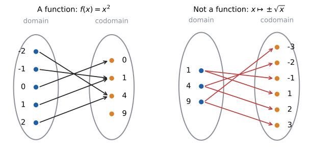
Notice what the right-hand picture says. "Give me a number whose square is 9" has two honest answers, +3 and −3. A rule with two answers is a perfectly good relation, but it is not a function. This is exactly why mathematicians define \(\sqrt{9}\) to mean the non-negative root only, 3: they wanted the square root to be a function.
11.1.3. Vocabulary and notation
|
Function
A function \(f\) from a set \(A\) to a set \(B\) is a rule that assigns to each element of \(A\) exactly one element of \(B\). We write \(f : A \to B\), read "\(f\) maps \(A\) to \(B\)" or "\(f\) from \(A\) to \(B\)". The arrow is about the whole function; it says where inputs come from and where outputs live. |
|
Input, output, argument, value, image
If \(f\) sends \(x\) to \(y\), we write \(f(x) = y\), read "\(f\) of \(x\) equals \(y\)".
The parentheses in \(f(x)\) mean "apply \(f\) to", not multiplication. \(f(x)\) is one object, the output. |
|
The "maps to" arrow and membership
\(x \mapsto x^2\) (a barred arrow) reads "\(x\) maps to \(x^2\)". It describes what happens to a single input, and lets you talk about a function without naming it. Compare:
\(x \in A\) reads "\(x\) is an element of \(A\)" (or "\(x\) is in \(A\)"). \(\mathbb{R}\) is the set of all real numbers, \(\mathbb{Z}\) the integers, \(\mathbb{N}\) the natural numbers (see Chapter 1). |
So "\(f : \mathbb{R} \to \mathbb{R},\ x \mapsto x^2\)" and "\(f(x) = x^2\) for real \(x\)" say the same thing; the first is the style of university texts, the second of school texts.
11.1.4. Worked example: evaluating a function
Let \(f(x) = 2x^2 - 3x + 1\). Find \(f(3)\), \(f(-1)\) and \(f(a+1)\).
The rule is "whatever is in the parentheses, put it everywhere you see \(x\)". Use brackets when substituting; they prevent sign errors.
Check with \(a = 2\): \(f(3)\) should equal \(2(2)^2 + 2 = 10\). It does.
|
\(f(x)\) is not \(f\) times \(x\)
Two classic errors come from treating \(f(\ldots)\) like multiplication:
Functions that do satisfy both rules are called linear maps. They are special, and they are the subject of Chapter 27. |
11.1.5. Four representations of one function
The same function can be shown in four ways, and fluency means moving between them freely:
| Representation | Example: the area of a square of side \(s\) |
|---|---|
Words |
"The area is the side length squared." |
Formula |
\(A(s) = s^2\), for \(s \ge 0\) |
Table |
\(s = 1, 2, 3, 4\) gives \(A = 1, 4, 9, 16\) |
Graph |
the right half of the parabola \(y = x^2\) |
A formula is compact and exact; a table is what a computer actually stores; a graph shows behaviour at a glance; words carry the meaning. None is "the" function. The function is the input-to-output assignment that all four describe.
|
Who invented "function"?
Leibniz used the word functio in the 1670s for quantities attached to a curve (such as its slope). Euler wrote \(f(x)\) in 1734 and for a long time meant "a formula". The modern definition (any rule, formula or not, that assigns one output per input) emerged in the 19th century with Dirichlet, who gave a famous example that no single formula could plausibly express: \(D(x) = 1\) if \(x\) is rational and \(0\) if irrational. The final step, defining a function as a set of input–output pairs, came with set theory around 1900. Programmers recover the same idea when they say "a function is just a lookup table with a very efficient compression scheme." |
11.2. Domain, codomain and range
11.2.1. The problem
Your code has a function sqrt(x). What happens if you call sqrt(-4)? In Python, math.sqrt(-4) raises ValueError: math domain error. The error message uses exactly the right mathematical word. Every function has a set of inputs it accepts, and asking for anything outside that set is meaningless (or, in the case of computers, an exception).
11.2.2. Vocabulary
|
Domain, codomain, range
For a function \(f : A \to B\):
Example: \(f : \mathbb{R} \to \mathbb{R},\ f(x) = x^2\). Domain \(\mathbb{R}\), codomain \(\mathbb{R}\), range \(\lbrack 0, \infty)\), since squares are never negative. |
The codomain versus range distinction is exactly the distinction between a function’s declared return type and the values it really returns. A Python function annotated → int that only ever returns 0 or 1 has codomain int and range \(\{0, 1\}\).
|
Interval notation and set-builder notation
Interval notation describes runs of real numbers. A square bracket includes the endpoint; a round bracket excludes it.
Set-builder notation \(\{x \in \mathbb{R} : x \ne 2\}\) reads "the set of real \(x\) such that \(x \ne 2\)". The colon (sometimes a vertical bar) means "such that". Python programmers already know this: |
11.2.3. Why domains get restricted
When a function is given by a formula with no domain stated, the convention is to use the natural domain: every real number for which the formula makes sense. In real-number algebra, only a few things can go wrong:
-
Division by zero. A denominator must not be zero.
-
Even roots of negatives. \(\sqrt{\ }\), \(\sqrt[4]{\ }\), … need a non-negative argument.
-
Logarithms of non-positives. \(\log(u)\) needs \(u > 0\) (you will meet this in Chapter 12).
A domain may also be restricted by the situation: a length cannot be negative, a number of people must be a whole number, a time might run only from launch to landing. These are called contextual or practical domains.
Input: a formula \(f(x)\).
Steps:
-
Start with all real numbers, \(\mathbb{R}\).
-
For every denominator, solve "denominator \(= 0\)" and remove those values.
-
For every even root, require "inside \(\ge 0\)" and solve the inequality.
-
For every logarithm, require "inside \(> 0\)" and solve.
-
Intersect all the conditions (an input must pass every test).
-
Write the result in interval notation.
Output: the natural domain of \(f\).
11.2.4. Worked examples
Example 1. \(g(x) = \dfrac{1}{x^2 - 4}\).
Denominator zero: \(x^2 - 4 = 0 \iff (x-2)(x+2) = 0 \iff x = \pm 2\). No roots or logs. Domain: \((-\infty, -2) \cup (-2, 2) \cup (2, \infty)\).
Example 2. \(f(x) = \dfrac{\sqrt{x - 3}}{x - 5}\).
Spot check: \(f(3) = 0/(-2) = 0\) is fine; \(f(5)\) would divide by zero; \(f(2)\) would need \(\sqrt{-1}\).
Example 3 (domain and range). \(h(x) = \sqrt{4 - x^2}\).
Domain: \(4 - x^2 \ge 0 \iff x^2 \le 4 \iff -2 \le x \le 2\), so \(\lbrack -2, 2]\).
Range: as \(x\) runs over \(\lbrack -2, 2]\), \(x^2\) runs over \(\lbrack 0, 4]\), so \(4 - x^2\) runs over \(\lbrack 0, 4]\) and its square root runs over \(\lbrack 0, 2]\). The range is \(\lbrack 0, 2]\). (The graph is the upper half of the circle of radius 2, which you can check against Chapter 10.)
11.2.5. Finding the range
Ranges are harder than domains; there is no universal recipe. Three methods cover most school cases:
-
Reason about pieces, as in Example 3: track what each operation does to a set of values.
-
Use a known graph. A parabola \(y = a(x - h)^2 + k\) with \(a > 0\) has range \(\lbrack k, \infty)\); with \(a < 0\), \((-\infty, k]\) (see Chapter 8).
-
Solve for \(x\). Set \(y = f(x)\) and ask: for which \(y\) does this equation have a solution \(x\) in the domain? Those \(y\) form the range.
Example of the third method: the range of \(f(x) = \dfrac{x - 1}{x - 2}\).
Every \(y \ne 1\) gives a valid \(x\) (and that \(x\) is never 2, because \(x = 2\) would need \(2y - 2 = 2y - 1\), impossible). So the range is \(\mathbb{R} \setminus \{1\}\). Hold on to this calculation: it is also how you find an inverse function, in Section 11.7.
|
Domain errors that hide inside simplification
\(\dfrac{x^2 - 1}{x - 1}\) simplifies to \(x + 1\), but the two are not the same function: the first is undefined at \(x = 1\); the second is not. Always find the domain from the original formula, before simplifying. The graph of the first is the line \(y = x + 1\) with a single missing point (a "hole") at \((1, 2)\). We return to holes in Section 11.9. |
11.3. Graphs and the vertical line test
11.3.1. The problem
A table of values shows a few points. A formula hides behaviour inside algebra. The graph shows everything at once: where the function is positive, where it rises, where it turns, where it is undefined. How do you know whether a curve someone draws is the graph of a function at all?
11.3.2. Vocabulary
|
Graph of a function
The graph of \(f\) is the set of all points \((x, f(x))\) for \(x\) in the domain. In set-builder form: \(\{(x, y) : x \in \text{domain},\ y = f(x)\}\). So "the point \((a, b)\) is on the graph" means exactly "\(f(a) = b\)". Reading a graph is evaluating a function with your eyes: go along to \(x = a\), then up or down to the curve, and read off the height. |
|
Intercepts, zeros and roots
|
11.3.3. The vertical line test
Since each input \(x\) has exactly one output, the graph contains exactly one point above (or below) each \(x\) in the domain, and none above \(x\) values outside it. A vertical line is the set of all points with a fixed \(x\), so:
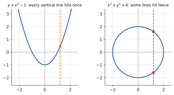
The circle is still a perfectly good curve, described by an equation in \(x\) and \(y\). It just is not the graph of one function of \(x\). Solving for \(y\) gives \(y = \pm\sqrt{4 - x^2}\): two functions, the upper semicircle \(y = \sqrt{4 - x^2}\) (Example 3 above) and the lower semicircle \(y = -\sqrt{4 - x^2}\). Splitting a curve into function-pieces like this is a routine move in calculus.
11.3.4. Reading a graph: what to look for
When you meet the graph of a new function, ask in this order:
-
Domain and range. What horizontal and vertical extent does it cover? Any gaps?
-
Intercepts. Where does it cross the axes?
-
Sign. Where is it above the \(x\)-axis (positive), where below (negative)?
-
Direction. Where does it rise, where fall? Where does it turn? (See Section 11.8.)
-
Symmetry. Is it mirror-symmetric about the \(y\)-axis, or symmetric under a half turn about the origin?
-
Ends and breaks. What happens as \(x \to \pm\infty\)? Are there asymptotes or holes (Section 11.9)?
|
Draw-and-test
Sketch any curve freehand on a coordinate grid. A vertical line follows the cursor and lights red whenever it meets the curve more than once; the app then offers to split the curve into the fewest function-pieces. Try a circle, a sideways parabola \(x = y^2\), and the letter S. |
11.4. Families of functions
11.4.1. The problem
There are infinitely many functions, but a small number of families do most of the work in science and computing. If you know the shape of each family’s basic member (its parent function), you can sketch almost anything by shifting and stretching (the next section). This section is a field guide.
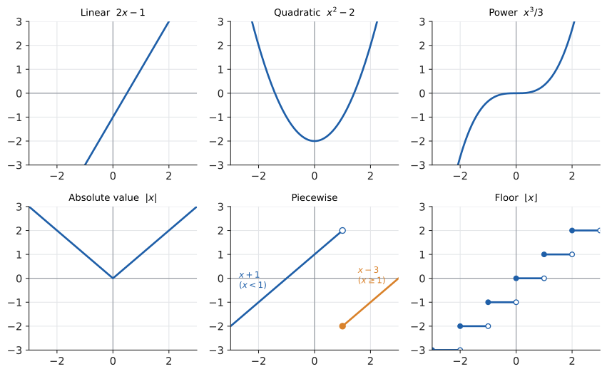
11.4.2. Linear functions
\(f(x) = mx + b\). Graph: a straight line with slope \(m\) and \(y\)-intercept \(b\) (all developed in Chapter 5). The defining property: equal steps in \(x\) give equal steps in \(y\). Increasing \(x\) by 1 always adds \(m\). Linear functions model anything with a constant rate: a taxi’s per-kilometre charge, a constant-speed journey, a linear cost.
11.4.3. Quadratic functions
\(f(x) = ax^2 + bx + c\) with \(a \ne 0\). Graph: a parabola, opening up if \(a > 0\) and down if \(a < 0\), with a vertex at \(x = -b/(2a)\) (see Chapter 8). Here equal steps in \(x\) give linearly growing steps in \(y\): for \(x^2\) the outputs 0, 1, 4, 9, 16 have differences 1, 3, 5, 7. Projectiles, areas, and the running time of a double loop are quadratic.
11.4.4. Power functions
\(f(x) = x^n\) (or \(kx^n\)). The shape depends on \(n\):
-
Even positive \(n\) (2, 4, 6, …): U-shaped, symmetric about the \(y\)-axis, range \(\lbrack 0, \infty)\). Higher powers are flatter near 0 and steeper beyond \(\lvert x \rvert = 1\).
-
Odd positive \(n\) (1, 3, 5, …): S-shaped through the origin, range \(\mathbb{R}\).
-
\(n = -1\): the reciprocal function \(1/x\), two separate branches, undefined at 0 (see Section 11.9).
-
\(n = 1/2\): the square root function \(\sqrt{x}\), domain and range \(\lbrack 0, \infty)\), the right half of a sideways parabola.
Power laws appear everywhere: \(A = \pi r^2\), \(V = \tfrac{4}{3}\pi r^3\), gravity proportional to \(r^{-2}\), algorithm costs \(n^2\), \(n^3\).
11.4.5. Absolute value
|
Absolute value function
\[\lvert x \rvert = \begin{cases} x & \text{if } x \ge 0\\ -x & \text{if } x < 0\end{cases}\]
It is the distance from \(x\) to 0 on the number line, so it is never negative. \(\lvert x - a \rvert\) is the distance between \(x\) and \(a\). The graph is a V with its corner at the origin. |
The definition above is our first piecewise formula, and the "\(-x\)" branch is the one that surprises people: if \(x = -3\) then \(-x = 3\). The minus sign makes a negative number positive.
11.4.6. Piecewise functions
|
Piecewise function
A piecewise function uses different formulas on different parts of its domain:
\[f(x) = \begin{cases} x + 1 & \text{if } x < 1\\ x - 3 & \text{if } x \ge 1\end{cases}\]
The big brace is read "\(f(x)\) equals \(x + 1\) if \(x < 1\), and \(x - 3\) if \(x \ge 1\)". The conditions must not overlap (else some \(x\) would get two outputs) and together should cover the whole domain. On a graph, a filled dot shows an endpoint that belongs to a piece; an open dot shows one that does not. |
The example above jumps at \(x = 1\): approaching from the left, the values approach 2; at \(x = 1\) itself, the value is \(1 - 3 = -2\). A jump like this is a discontinuity, a concept made precise in Chapter 16.
Piecewise functions are just if/elif/else written in mathematics. Every function in your code with a branch is piecewise.
11.4.7. Step functions: floor, ceiling and rounding
|
Floor and ceiling
\(\lfloor 3.7 \rfloor = 3\), \(\lceil 3.2 \rceil = 4\), \(\lfloor 5 \rfloor = \lceil 5 \rceil = 5\). Careful with negatives: \(\lfloor -3.5 \rfloor = -4\) (down means towards \(-\infty\), not towards 0), and \(\lceil -3.5 \rceil = -3\). These are step functions: their graphs are flat stairs with a jump at each integer. |
|
Floor is not truncation
"Chop off the decimals" (truncation, rounding towards zero) agrees with floor for positive numbers and with ceiling for negative numbers. Languages disagree about which one integer division uses. Python’s |
import math

def pages_needed(n_items, per_page):
    return math.ceil(n_items / per_page)

print(pages_needed(95, 10), pages_needed(100, 10), pages_needed(101, 10))
print(7 // 2, -7 // 2, int(-7 / 2))        # floor vs truncation
print(math.floor(-3.5), math.ceil(-3.5), round(2.5), round(3.5))
10 10 11 3 -4 -3 -4 -3 2 4
11.4.8. Where you’d use this
-
Linear: a plumber charges a $60 call-out fee plus $45 an hour: \(C(t) = 60 + 45t\), so a 2.5-hour job is \(60 + 112.5 = \$172.50\).
-
Quadratic: braking distance grows with the square of speed. The UK Highway Code gives a braking distance of 14 m at 30 mph and 55 m at 60 mph: double the speed, roughly four times the distance (\(55/14 \approx 3.9\)). The thinking distance (9 m and 18 m) is linear in speed, so total stopping distance is a quadratic plus a linear term.
-
Power: light, sound and gravity all follow an inverse-square law, \(I = k/r^2\). Move a lamp from 1 m to 2 m away from your book and the light on the page falls to \(1/2^2 = 1/4\) of what it was; to 3 m, \(1/9\).
-
Absolute value: engineering tolerances are absolute-value inequalities. A shaft specified as \(25.00 \pm 0.05\) mm passes inspection when \(\lvert d - 25.00 \rvert \le 0.05\). In statistics and machine learning, the mean absolute error averages \(\lvert \text{prediction} - \text{truth} \rvert\).
-
Piecewise: a thermostat (heating on below 19 °C, off above 21 °C), income tax bands (Section 11.10), and the most common function in deep learning, the ReLU \(\operatorname{ReLU}(x) = \max(0, x)\), which is \(0\) for \(x < 0\) and \(x\) for \(x \ge 0\). A neural network built from ReLUs is one enormous piecewise-linear function.
-
Step: postage by weight band, car-park charges "per hour or part hour", phone-data bundles, and every pagination or bucket count in code (the CS sidebar above).
11.4.9. Choosing a family
When you have data or a description and need a model, the family is chosen by how the output changes when the input changes:
| Pattern of change | Family | Typical example |
|---|---|---|
Constant additive change per step |
Linear |
hourly wages |
Additive change that itself grows steadily |
Quadratic |
distance fallen, double loops |
Doubling or halving per step |
Exponential (Chapter 12) |
compound interest, cell growth |
Scaling input by \(k\) scales output by \(k^n\) |
Power |
area and volume vs length |
Different rules on different ranges |
Piecewise |
tax, shipping, thermostats |
Flat, then sudden jumps |
Step |
postage, pagination |
Repeating |
Periodic (Chapter 13) |
seasons, waves, clocks |
|
Family portraits
Choose a family and drag sliders for its parameters (\(m, b\) for lines, \(a, b, c\) for quadratics, \(k, n\) for powers). A second panel shows the table of values and its first and second differences, so you can see "constant first differences = linear, constant second differences = quadratic" happening live. Try it: Quadratic family with table |
11.5. Transformations of graphs
11.5.1. The problem
You know the graph of \(y = x^2\). What does \(y = -2(x - 3)^2 + 4\) look like? Or \(y = \lvert 2x + 6 \rvert - 1\)? You could plot a table of points each time, but there is a far better way: every one of these is the parent graph moved and stretched, and the formula tells you exactly how.
11.5.2. Intuition: four moves
Start with a function \(f\) whose graph you know. There are four basic changes, two to the output and two to the input:
| Formula | Change | Effect on graph |
|---|---|---|
\(f(x) + k\) |
add to output |
shift up by \(k\) |
\(a \cdot f(x)\) |
multiply output |
stretch vertically by factor \(a\); if \(a < 0\), also reflect in the \(x\)-axis |
\(f(x - h)\) |
subtract from input |
shift right by \(h\) |
\(f(bx)\) |
multiply input |
squeeze horizontally by factor \(b\) (stretch by \(1/b\)); if \(b < 0\), also reflect in the \(y\)-axis |
The output changes do what you expect. The input changes feel backwards: \(x - 3\) moves the graph right, and \(2x\) makes it narrower. Why?
11.5.3. Why it works: the input changes are "backwards"
Let \(g(x) = f(x - 3)\). Ask: where does \(g\) do what \(f\) does at 0? That is, when is the input to \(f\) equal to 0? When \(x - 3 = 0\), so at \(x = 3\). Everything \(f\) did at 0, \(g\) does at 3; everything \(f\) did at 1, \(g\) does at 4. The whole graph has moved 3 to the right. The subtraction is the delay: \(g\) has to wait until \(x\) reaches 3 before it gets the input 0.
Similarly, let \(g(x) = f(2x)\). When is the input to \(f\) equal to 6? When \(2x = 6\), so at \(x = 3\). \(g\) gets through \(f\)'s inputs twice as fast, so its graph is squashed horizontally by a factor of 2.
The rule of thumb: changes outside \(f\) act on \(y\) directly; changes inside \(f\) act on \(x\) inversely. To find where a point goes, solve "inside = old input" for \(x\).
11.5.4. The general rule
All four moves combine into one formula:
If \((x_0, y_0)\) is on the graph of \(f\), then the corresponding point on the graph of \(g\) is where the input to \(f\) is again \(x_0\):
On the \(x\) side: scale by \(1/b\), then shift by \(h\). On the \(y\) side: scale by \(a\), then shift by \(k\). In each direction, scale first, then shift.
Input: a parent function \(f\) with known graph; a formula for \(g\).
Steps:
-
Rewrite the inside in the form \(b(x - h)\) by factoring out the coefficient of \(x\). (\(f(2x - 6)\) becomes \(f(2(x - 3))\), so \(h = 3\), not 6.)
-
Read off \(a, b, h, k\). Write \(x + 3\) as \(x - (-3)\), so \(h = -3\).
-
Choose 3–5 easy key points \((x_0, y_0)\) on the parent (vertex, intercepts, corners).
-
Map each with \((x_0, y_0) \mapsto (x_0/b + h,\ a y_0 + k)\).
-
Plot the new points and draw the parent shape through them.
-
Check by evaluating \(g\) directly at one point.
Output: a sketch of \(g\) and its key points.
11.5.5. Worked example 1: a reshaped parabola
Sketch \(g(x) = -2(x - 3)^2 + 4\). Try it: Graph g(x) = −2(x − 3)² + 4.
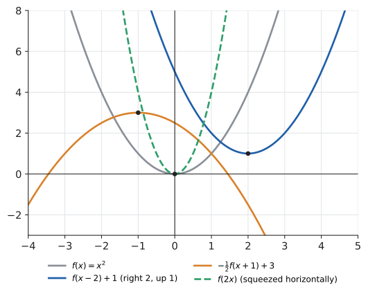
Parent: \(f(x) = x^2\). Here \(a = -2\), \(b = 1\), \(h = 3\), \(k = 4\). Key points on the parent: \((-1, 1), (0, 0), (1, 1), (2, 4)\).
So: a parabola opening down (since \(a < 0\)), twice as steep as \(x^2\), with vertex \((3, 4)\). Check directly: \(g(5) = -2(2)^2 + 4 = -8 + 4 = -4\). Correct. This is exactly the vertex form of a quadratic from Chapter 8; now you can see that vertex form is the transformation rule.
11.5.6. Worked example 2: a horizontal squeeze in disguise
Sketch \(g(x) = \lvert 2x + 6 \rvert - 1\). Try it: Graph g(x) = |2x + 6| − 1.
Step 1, factor the inside: \(2x + 6 = 2(x + 3) = 2(x - (-3))\). So \(a = 1\), \(b = 2\), \(h = -3\), \(k = -1\). Parent key points of \(\lvert x \rvert\): \((-2, 2), (0, 0), (2, 2)\).
A V with its corner at \((-3, -1)\), with sides of slope \(\pm 2\). Check: \(g(-2) = \lvert 2 \rvert - 1 = 1\). Correct.
def transform(points, a=1, b=1, h=0, k=0):
    """Image of points on y=f(x) under y = a*f(b(x-h)) + k."""
    return [(x / b + h, a * y + k) for x, y in points]

base = [(-1, 1), (0, 0), (1, 1), (2, 4)]       # points on y = x^2
print(transform(base, a=-2, b=1, h=3, k=4))
print(transform(base, b=2))
[(2.0, 2), (3.0, 4), (4.0, 2), (5.0, -4)] [(-0.5, 1), (0.0, 0), (0.5, 1), (1.0, 4)]
|
Shift by \(h\), not by the constant
|
11.5.7. Where you’d use this
The four moves have everyday meanings once the input is time:
-
\(f(t - h)\) is a delay. If \(f(t)\) is the temperature in London at time \(t\) (hours), a city whose weather pattern arrives 3 hours later sees \(f(t - 3)\). An echo of a sound \(f(t)\) arriving 0.25 s later at 30% of the volume is \(0.3\,f(t - 0.25)\); audio software builds reverb by adding many such copies.
-
\(f(bt)\) is a speed change. Playing a video at 2× speed shows \(f(2t)\): everything happens at half the time. (Played back at 2× without correction, audio frequencies double too, which is why sped-up voices sound squeaky.)
-
\(a f(t) + k\) is a change of units or calibration. Converting a temperature graph from Celsius to Fahrenheit is \(1.8 f(t) + 32\): a vertical stretch by 1.8 and a shift up by 32. A bathroom scale that reads 0.5 kg heavy needs \(f - 0.5\).
In science, recognising a transformed parent saves work: once you know the shape of \(y = x^2\), you know the shape of every projectile path, and once you know \(1/x\) you know Boyle’s law (\(P = k/V\)) for every gas sample.
|
Four sliders
Pick a parent (\(x^2\), \(\lvert x \rvert\), \(\sqrt{x}\), \(x^3\), \(\lfloor x \rfloor\)) and drag sliders for \(a, b, h, k\) in \(a f(b(x - h)) + k\). Ghost arrows show where each key point of the parent goes. Then try "guess the formula": the app shows a transformed graph and you set the sliders to match it. Try it: a f(b(x − h)) + k sliders |
11.6. Composition: functions in a pipeline
11.6.1. The problem
A shop converts a price in dollars to euros, then adds 20% tax. Converting is one function; adding tax is another. The whole process (dollars in, final euro price out) is a third function made by running the first, then feeding its output into the second. That is composition, and it is how complicated functions are built from simple ones.
11.6.2. Vocabulary
|
Composition of functions
The composition of \(f\) and \(g\) is the function \(f \circ g\), read "\(f\) composed with \(g\)", "\(f\) after \(g\)", or "\(f\) of \(g\)":
\[(f \circ g)(x) = f\big(g(x)\big)\]
Order: \(g\) is applied first, even though it is written second. Read \(f \circ g\) from right to left, like nested function calls \(f \circ g\) is defined at \(x\) only when \(x\) is in the domain of \(g\) and \(g(x)\) is in the domain of \(f\). |
11.6.3. Worked example 1: order matters
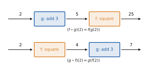
Let \(f(x) = x^2\) and \(g(x) = x + 3\).
At \(x = 2\): \((f \circ g)(2) = 25\) but \((g \circ f)(2) = 7\). "Add 3 then square" is not "square then add 3". Composition is not commutative. (It is, however, associative: \(f \circ (g \circ h) = (f \circ g) \circ h\), both meaning "do \(h\), then \(g\), then \(f\)".)
11.6.4. Worked example 2: the domain of a composition
Let \(f(x) = \sqrt{x}\) and \(g(x) = x - 4\).
-
\((f \circ g)(x) = \sqrt{x - 4}\). Need \(g(x) = x - 4 \ge 0\), so the domain is \(\lbrack 4, \infty)\).
-
\((g \circ f)(x) = \sqrt{x} - 4\). Need \(x \ge 0\) for the root; then subtracting 4 is always fine. Domain \(\lbrack 0, \infty)\).
A subtler case: with \(p(x) = x^2\) and \(q(x) = \sqrt{x}\), \((p \circ q)(x) = (\sqrt{x})^2 = x\). The simplified formula \(x\) looks defined everywhere, but \(p \circ q\) is defined only for \(x \ge 0\), because \(q\) must be able to act first. As with holes, find the domain before simplifying.
11.6.5. Decomposition
Often the useful move is the reverse: seeing a complicated function as a composition of simple ones.
\(h(x) = (3x - 1)^5\) is \(f(g(x))\) with inner function \(g(x) = 3x - 1\) and outer function \(f(u) = u^5\).
\(k(x) = \sqrt{x^2 + 1}\) is \(f(g(x))\) with \(g(x) = x^2 + 1\) and \(f(u) = \sqrt{u}\).
The question to ask is "what would I compute last on a calculator?" That is the outer function. This skill is exactly what the chain rule needs in Chapter 17, where the derivative of a composition is built from the derivatives of the pieces.
The transformation rule of the last section is itself a composition: \(a f(b(x - h)) + k\) is "subtract \(h\), multiply by \(b\), apply \(f\), multiply by \(a\), add \(k\)", a five-stage pipeline.
11.6.6. Where you’d use this
-
Shopping. The opening problem with numbers: convert dollars to euros at 0.92, then add 20% tax. A $50 item becomes \(50 \times 0.92 = 46\) euros, then \(46 \times 1.2 = 55.20\) euros. Here the order doesn’t matter (both steps are multiplications), but with a 10%-off sale and a $5 coupon it does: discount then coupon gives \(0.9 \times 50 - 5 = \$40.00\); coupon then discount gives \(0.9 \times (50 - 5) = \$40.50\). Shops choose the order, and now you know to check.
-
Science. Unit conversions chain: km/h to m/s (divide by 3.6), then m/s to kinetic energy per kilogram (\(v \mapsto \tfrac12 v^2\)). A sensor reading passes through calibration, filtering and conversion before it reaches a screen; each stage is a function, and the whole instrument is their composition.
-
Machine learning. A neural network is a long composition: layer 1, then layer 2, …, each a simple function. Training it uses the chain rule (Chapter 17), which is precisely "how does a composition change when its pieces change?"
11.7. Inverse functions
11.7.1. The problem
Fahrenheit from Celsius is \(F = \tfrac{9}{5}C + 32\). A visitor wants the other direction: given \(F\), what is \(C\)? We want a function that undoes the first one. When does such an undo function exist, and how do you find it?
11.7.2. Intuition: run the machine backwards
In the mapping picture, inverting a function means reversing every arrow. For the result to be a function again, two things must hold:
-
No output may receive two arrows; otherwise, reversed, it would send out two arrows. (Squaring fails: 4 receives arrows from both 2 and −2, so "un-squaring 4" is ambiguous.)
-
Every element of the codomain should receive an arrow; otherwise, reversed, it would send out none. (This is often fixed simply by shrinking the codomain to the range.)
|
One-to-one and inverse
A function is one-to-one (or injective) if different inputs always give different outputs: \(x_1 \ne x_2 \Rightarrow f(x_1) \ne f(x_2)\). Equivalently, \(f(x_1) = f(x_2) \Rightarrow x_1 = x_2\). If \(f\) is one-to-one with range \(R\), its inverse function \(f^{-1} : R \to \text{domain of } f\) is defined by
\[f^{-1}(y) = x \iff f(x) = y.\]
Read \(f^{-1}\) as "\(f\) inverse". The inverse undoes \(f\) and vice versa: \(f^{-1}(f(x)) = x\) for every \(x\) in the domain of \(f\), and \(f(f^{-1}(y)) = y\) for every \(y\) in its range. In composition notation, \(f^{-1} \circ f\) and \(f \circ f^{-1}\) are identity functions. The domain and range swap roles. |
|
\(f^{-1}\) is not \(1/f\)
The superscript \(-1\) on a function name means inverse function, not reciprocal. If \(f(x) = 2x\), then \(f^{-1}(x) = x/2\) but \(1/f(x) = 1/(2x)\). The notation is borrowed from composition: just as \(a^{-1} a = 1\), \(f^{-1} \circ f = \text{identity}\). To make matters worse, trigonometry uses \(\sin^2 x\) to mean \((\sin x)^2\) while \(\sin^{-1} x\) means the inverse sine; Chapter 13 deals with that. |
11.7.3. The horizontal line test
On a graph, "two inputs with the same output" means two points at the same height. So:
Lines with nonzero slope pass. \(x^3\) passes. \(x^2\) fails (the line \(y = 4\) meets it at \(x = \pm 2\)), as does \(\lvert x \rvert\). Any function that is strictly increasing or strictly decreasing everywhere on its domain passes automatically (see Section 11.8).
11.7.4. Why the graph reflects in \(y = x\)
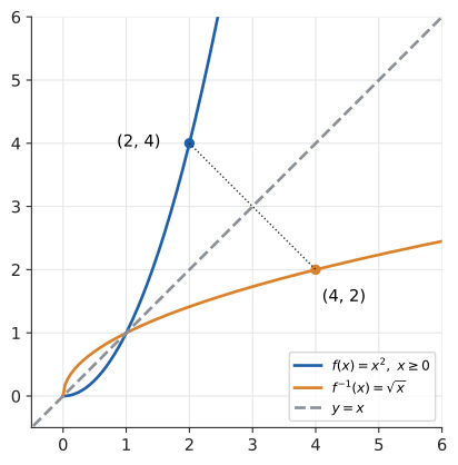
If \((a, b)\) is on the graph of \(f\), then \(f(a) = b\), so \(f^{-1}(b) = a\), so \((b, a)\) is on the graph of \(f^{-1}\). Swapping the coordinates of every point is the same as reflecting the plane in the line \(y = x\). The graph of \(f^{-1}\) is the mirror image of the graph of \(f\) in the line \(y = x\).
11.7.5. Restricting the domain
\(x^2\) on all of \(\mathbb{R}\) has no inverse. But on the restricted domain \(\lbrack 0, \infty)\) it is one-to-one, and its inverse is \(\sqrt{x}\). On \((-\infty, 0]\) it is also one-to-one, with inverse \(-\sqrt{x}\). The square root function exists because we chose the right half. The same choice gives the inverse trigonometric functions in Chapter 13, and the logarithm is the inverse of the exponential (which needs no restriction) in Chapter 12.
Input: a formula \(y = f(x)\).
Steps:
-
Check that \(f\) is one-to-one (horizontal line test, or monotonicity). If not, restrict the domain.
-
Write \(y = f(x)\).
-
Solve the equation for \(x\) in terms of \(y\). (Note any values of \(y\) for which this is impossible: they are outside the range.)
-
Swap the letters \(x\) and \(y\) if you want the inverse written as a function of \(x\). Name it \(f^{-1}(x)\).
-
State the domain of \(f^{-1}\) (the range of \(f\)).
-
Check with a number: pick \(a\), compute \(b = f(a)\), and confirm \(f^{-1}(b) = a\).
Output: \(f^{-1}\) with its domain.
Some books swap \(x\) and \(y\) first and then solve; the two orders are equivalent. Solving first keeps the meaning clearer ("given the output, recover the input"), which matters in applications where \(x\) and \(y\) stand for different quantities like Celsius and Fahrenheit.
11.7.6. Worked example 1: a linear function
Find the inverse of \(f(x) = \dfrac{2x + 3}{5}\).
Check: \(f(6) = (12 + 3)/5 = 3\), and \(f^{-1}(3) = (15 - 3)/2 = 6\). Correct. Notice the inverse undoes the steps in reverse order: \(f\) multiplies by 2, adds 3, divides by 5; \(f^{-1}\) multiplies by 5, subtracts 3, divides by 2. Like taking off socks and shoes: the last thing on is the first thing off. In symbols, \((f \circ g)^{-1} = g^{-1} \circ f^{-1}\).
For Celsius and Fahrenheit, the same steps turn \(F = \tfrac{9}{5}C + 32\) into \(C = \tfrac{5}{9}(F - 32)\).
11.7.7. Worked example 2: a rational function
Find the inverse of \(f(x) = \dfrac{3x + 1}{x - 2}\), \(x \ne 2\).
The range of \(f\) is everything except 3, which becomes the domain of \(f^{-1}\). Check: \(f(3) = 10/1 = 10\); \(f^{-1}(10) = 21/7 = 3\). Correct.
11.7.8. Alternative approaches and choosing a method
-
Reverse the steps (as in the socks-and-shoes remark). Fastest when \(x\) appears once in the formula: list the operations applied to \(x\), then undo them in reverse order.
-
Solve for \(x\) (the procedure). Needed when \(x\) appears more than once, as in Example 2: gather the \(x\) terms and factor.
-
Graphically, reflect in \(y = x\). Useful for sketching, not for formulas.
-
Numerically, when no formula exists. If \(f\) is increasing, you can find \(f^{-1}(y)\) by bisection: search for the \(x\) with \(f(x) = y\) the way binary search finds a key (Chapter 32). This is how many libraries compute inverses of complicated functions.
11.7.9. Where you’d use this
-
Working backwards from a target. At 5% interest, money grows as \(A = 1.05P\) in a year. To have $1,000 next year you need the inverse: \(P = A/1.05 = 1000/1.05 \approx \$952.38\) today. "How much do I need to start with?" is always an inverse-function question.
-
Accident investigation. A car braking with friction coefficient \(\mu\) skids a distance \(d = v^2/(2\mu g)\) from speed \(v\) (a mechanics result). Police reconstructing a crash measure the skid and invert: \(v = \sqrt{2\mu g d}\). With \(\mu = 0.7\), \(g = 9.81\) m/s² and a 30 m skid, \(v = \sqrt{2(0.7)(9.81)(30)} \approx 20.3\) m/s, about 73 km/h. The formula needs \(v \ge 0\): the restriction to the right half of the parabola, exactly as with \(\sqrt{x}\).
-
Measurement in general. Instruments measure one thing and report another: a thermometer measures expansion, a GPS measures signal delay, a camera measures light. Turning the raw reading back into the quantity you want is applying an inverse function, and it only works if the original was one-to-one over the range in use.
|
Mirror in \(y = x\)
Draw a function’s graph; the app draws its reflection in \(y = x\) and colours it red wherever the reflection fails the vertical line test. Drag a "domain window" to restrict the original until the reflection becomes a valid function. Try it: Reflect y = x² in y = x |
11.8. Symmetry and direction: even, odd, increasing, decreasing
11.8.1. The problem
Some graphs have a symmetry you can exploit: compute half, get the other half free. Others always go up, which guarantees an inverse exists and allows binary search. These properties can be tested algebraically, without drawing.
11.8.2. Even and odd functions
|
Even and odd functions
Most functions are neither. The names come from powers: \(x^n\) is even exactly when \(n\) is even, and odd when \(n\) is odd. |
Worked example. Classify \(f(x) = x^4 - 3x^2\), \(g(x) = x^3 + x\), \(h(x) = x^2 + x\).
For \(h\), the result \(x^2 - x\) is neither \(h(x) = x^2 + x\) nor \(-h(x) = -x^2 - x\) (try \(x = 1\): \(h(-1) = 0\) while \(h(1) = 2\)). So \(h\) is neither even nor odd. One counterexample is enough to rule a property out; to establish it, you need the algebra for all \(x\).
def parity(f, samples=(0.5, 1, 2, 3.7)):
    even = all(abs(f(-x) - f(x)) < 1e-12 for x in samples)
    odd = all(abs(f(-x) + f(x)) < 1e-12 for x in samples)
    return "even" if even else "odd" if odd else "neither"

print(parity(lambda x: x**4 - 3*x**2))
print(parity(lambda x: x**3 + x))
print(parity(lambda x: x**2 + x))
even odd neither
|
Sampling is evidence, not proof
The |
|
Every function is even plus odd
Any function defined on a symmetric domain splits uniquely into an even part and an odd part:
\[f(x) = \underbrace{\frac{f(x) + f(-x)}{2}}_{\text{even}} + \underbrace{\frac{f(x) - f(-x)}{2}}_{\text{odd}}\]
For a polynomial, this just separates even and odd powers. For \(e^x\) it produces the hyperbolic cosine and sine, \(\cosh x\) and \(\sinh x\), which describe the shape of a hanging chain. The same splitting idea, generalised, is the start of Fourier analysis. |
11.8.3. Increasing and decreasing
|
Increasing, decreasing, monotonic
On an interval \(I\):
Some books say "strictly increasing" for this and "increasing" or "non-decreasing" for the version with \(\le\). A local maximum is a point higher than all nearby points; a local minimum, lower. They occur where a function switches between increasing and decreasing. |
Example: \(f(x) = x^2\) is decreasing on \((-\infty, 0]\) and increasing on \(\lbrack 0, \infty)\), with a minimum at 0. The parabola \(-2(x - 3)^2 + 4\) is increasing on \((-\infty, 3]\), decreasing on \(\lbrack 3, \infty)\), with a maximum of 4 at \(x = 3\).
Two important facts:
-
A strictly monotonic function is one-to-one, and therefore has an inverse. (If \(x_1 \ne x_2\), one is smaller, so their outputs differ.) This is why the restriction of \(x^2\) to \(\lbrack 0, \infty)\) works.
-
Finding where a function increases and decreases, for functions you cannot just picture, is one of the main jobs of the derivative (Chapter 18).
11.9. Rational functions and asymptotes: a first look
11.9.1. The problem
The average cost per item of a print run, with a fixed setup cost of $500 and $2 per copy, is \(C(n) = \dfrac{500 + 2n}{n}\). For small runs the cost is enormous; for huge runs it settles towards $2 but never gets there. Graphs like this, which blow up near some inputs and level off far away, belong to rational functions.
|
Rational function and asymptote
A rational function is a quotient of two polynomials, \(R(x) = \dfrac{P(x)}{Q(x)}\), with \(Q\) not the zero polynomial (the name comes from ratio, as with rational numbers). Its natural domain is every real number except the zeros of \(Q\). An asymptote is a line that the graph approaches ever more closely:
"\(x \to \infty\)" reads "as \(x\) grows without bound". The precise language for "gets as close as you like" is the limit, defined in Chapter 16. |
11.9.2. Intuition: the reciprocal function
The parent is \(y = 1/x\). Near \(x = 0\), dividing 1 by a tiny number gives a huge number: \(1/0.001 = 1000\), \(1/(-0.001) = -1000\). So the graph shoots up on the right of 0 and down on the left: a vertical asymptote at \(x = 0\). Far out, dividing 1 by a huge number gives almost 0: a horizontal asymptote at \(y = 0\).
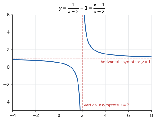
Now use transformations. \(y = \dfrac{1}{x - 2} + 1\) is \(1/x\) shifted right 2 and up 1, so its asymptotes are \(x = 2\) and \(y = 1\). And that is the function from the range example, since
This explains, geometrically, why its range was everything except 1.
11.9.3. The method
Input: a rational function \(R(x) = P(x)/Q(x)\).
Steps:
-
Factor \(P\) and \(Q\) completely (see Chapter 7).
-
Holes: for each factor \((x - a)\) common to \(P\) and \(Q\), cancel it; the graph has a hole at \(x = a\). Its \(y\)-coordinate is the cancelled formula evaluated at \(a\).
-
Vertical asymptotes: after cancelling, each remaining zero \(a\) of the denominator gives a vertical asymptote \(x = a\).
-
Horizontal asymptote: compare degrees \(\deg P\) and \(\deg Q\):
-
\(\deg P < \deg Q\): \(y = 0\);
-
\(\deg P = \deg Q\): \(y = \dfrac{\text{leading coefficient of } P}{\text{leading coefficient of } Q}\);
-
\(\deg P > \deg Q\): no horizontal asymptote (if \(\deg P = \deg Q + 1\) there is a slanted, or oblique, asymptote, found by polynomial division).
-
Output: holes, vertical asymptotes, and the horizontal (or oblique) asymptote.
Why the degree rule works. Far from the origin, the highest power dominates each polynomial. For \(R(x) = \dfrac{2x^2 + 1}{x^2 - 9}\), divide top and bottom by \(x^2\):
11.9.4. Worked example
Analyse \(R(x) = \dfrac{2x^2 + 1}{x^2 - 9}\).
-
Factor: \(2x^2 + 1\) does not factor over the reals (it is always positive); \(x^2 - 9 = (x - 3)(x + 3)\).
-
No common factors, so no holes.
-
Vertical asymptotes: \(x = 3\) and \(x = -3\).
-
Degrees equal (2 and 2): horizontal asymptote \(y = 2/1 = 2\).
Also: \(R(0) = 1/(-9) = -1/9\) (the \(y\)-intercept), and since the numerator is never zero there are no \(x\)-intercepts. \(R\) is even, since only even powers appear.
A hole. \(S(x) = \dfrac{x^2 - 1}{x - 1} = \dfrac{(x - 1)(x + 1)}{x - 1}\). The factor \(x - 1\) cancels, so there is a hole at \(x = 1\), at height \(1 + 1 = 2\), and no vertical asymptote. The graph is the line \(y = x + 1\) with the point \((1, 2)\) removed.
For the print-run example, \(C(n) = (500 + 2n)/n\) has equal degrees, leading coefficients 2 and 1, so the horizontal asymptote is \(y = 2\): the cost per copy approaches $2. Writing it as \(C(n) = 2 + 500/n\) makes that obvious: the setup cost is spread ever more thinly.
|
Asymptotes are not walls
|
11.9.5. Where you’d use this
-
Travel time. For a fixed 50 km trip, time is \(t(v) = 50/v\), the reciprocal shape. At 110 km/h it takes \(50/110 \times 60 \approx 27.3\) minutes; at 130 km/h, about 23.1 minutes. Driving 20 km/h faster saves only about 4 minutes, because the curve is flattening out. (Going from 30 to 50 km/h on the same trip would save 40 minutes.)
-
Physics and chemistry. Boyle’s law \(P = k/V\) (halve the volume of a gas, double its pressure), two resistors in parallel \(R = \dfrac{R_1 R_2}{R_1 + R_2}\), and the thin-lens equation are all rational functions; their vertical asymptotes are physically meaningful (a lens focusing at infinity, a short circuit).
-
Business. Any "fixed cost plus per-unit cost, divided by units" is the print-run curve. A $1,200 coffee machine that saves $3 a day pays for itself in 400 days; the average cost per cup keeps falling but never below the cost of the beans.
11.10. Functions as models
11.10.1. The problem
A function is also a claim about the world: "tax depends on income like this", "height depends on time like that". Building such a model means choosing variables, choosing a family, fitting parameters, and (the step most often skipped) stating the domain where the model is valid.
11.10.2. Worked example 1: a piecewise tax schedule
A (simplified, fictional) tax system: 10% on income up to $10,000, and 20% on every dollar above $10,000. Write tax \(T\) as a function of income \(x\) and compute \(T(25{,}000)\).
On the first $10,000 the tax is \(0.1x\). Above that, the first $10,000 contributes \(0.1 \times 10{,}000 = 1{,}000\), and the excess \(x - 10{,}000\) is taxed at 20%:
Check continuity at the boundary: the first branch gives \(T(10{,}000) = 1{,}000\), and the second branch, as \(x\) approaches 10,000 from above, approaches \(1{,}000 + 0 = 1{,}000\). No jump. That is the meaning of marginal rates: moving into a higher bracket only raises the tax on the extra dollars, so earning more never leaves you with less. (A system with a jump in tax at the boundary would create exactly that perverse effect, which is why real systems are designed as continuous piecewise-linear functions.)
11.10.3. Worked example 2: a step-function price
A courier charges $3.00 for the first kilogram (or part of one) and $1.50 for each additional kilogram or part. Model the cost and price a 2.3 kg parcel.
"Or part" means round up. A parcel of weight \(w\) counts as \(\lceil w \rceil\) kilograms, of which the first is charged at $3.00:
Sanity checks: \(C(0.4) = 3 + 1.5(1 - 1) = 3.00\); \(C(1) = 3.00\); \(C(1.01) = 3 + 1.5 = 4.50\).
11.10.4. Worked example 3: a projectile and its practical domain
A ball is thrown upwards from 1.5 m with speed 20 m/s. Ignoring air resistance, its height after \(t\) seconds is \(h(t) = -4.9t^2 + 20t + 1.5\) metres. What is the practical domain, the maximum height, and the range?
The model only makes sense from the throw (\(t = 0\)) until the ball lands (\(h(t) = 0\), \(t > 0\)). Using the quadratic formula (Chapter 8) on \(4.9t^2 - 20t - 1.5 = 0\):
(The other root is negative, before the throw, so we discard it.) The domain is \(\lbrack 0, 4.155]\) approximately.
The vertex is at \(t = -b/(2a) = -20/(2 \times -4.9) \approx 2.041\) s, and
So the range is about \(\lbrack 0, 21.9]\) metres. Outside the domain the formula still produces numbers (\(h(6) \approx -55\)), but they mean nothing: the ball does not burrow 55 m underground.
|
Extrapolation
A model fitted on data from one range of inputs can be badly wrong outside it. A straight line fitted to a child’s height from ages 2 to 10 predicts a 40-year-old over 3 m tall. Always state the domain of validity, and be suspicious of any prediction that leaves it. Machine-learning models have the same failure under the name distribution shift. |
|
Fit a family
Load a small data set (stopping distance against speed, average cost against batch size, height against time). Choose a family, drag its parameters to fit the points, and watch a residual plot. Then drag a slider extending the \(x\)-range beyond the data and see which fitted families stay sensible and which go wild. Try it: Fit braking distances |
11.11. Functions in computing
Programmers use the word "function" every day, and it means something close to, but not the same as, the mathematical idea. Knowing exactly where they differ makes you a better reader of mathematics and a better writer of code.
11.11.1. Mathematical functions versus programming functions
A mathematical function is only an input-to-output assignment. It does not "run", take time, print anything, or remember previous calls. A programming function (a subroutine, procedure or method) is a piece of code that may do all of those things.
|
Pure function and side effect
A programming function is pure if
A pure function is a mathematical function. Calling it twice with the same arguments must give the same result, so the call can always be replaced by its value (referential transparency). |
total = 0

def add_impure(x):
    global total          # reads and writes state outside itself
    total += x
    return total

def add_pure(acc, x):
    return acc + x        # output depends only on inputs

print(add_impure(5), add_impure(5))   # same input, different outputs
print(add_pure(0, 5), add_pure(0, 5)) # same input, same output
5 10 5 5
add_impure fails the defining property of a function: the input 5 produced two different outputs. Mathematically, it is a function of two inputs (the argument and the hidden state), and making that hidden input explicit, as add_pure does, is the standard repair. Functional programming is largely the discipline of making every input explicit.
Other differences worth knowing:
-
Partiality. Many program functions do not return for some inputs: they raise, loop forever, or crash. Mathematically these are partial functions (see Section 11.2).
-
Time and memory. Mathematics ignores how long a function takes; computer science studies exactly that (\(O(n^2)\) and friends).
-
Equality. Two mathematical functions are equal if they have the same domain and give the same output for every input, however differently they are computed. Bubble sort and merge sort compute the same function.
-
Floating point.
f(x)in code computes an approximation; \(0.1 + 0.2\) is not exactly \(0.3\) (see Chapter 32).
11.11.2. Functions as data: first-class functions
In mathematics, functions are objects you can pass around: composition takes two functions and returns a function; the derivative (Chapter 17) takes a function and returns a function. Languages with first-class functions allow the same: functions can be stored in variables, passed as arguments, and returned as results. A function that takes or returns functions is a higher-order function. compose, map, filter, sorted(key=…), and decorators are all higher-order. The Python lambda x: x ** 2 is a direct transcription of \(x \mapsto x^2\).
11.11.3. Lookup tables: a function is its table
Mathematically, a function on a finite domain is nothing more than its table of input–output pairs. Computing can trade time for space by storing that table:
from functools import lru_cache
calls = 0

@lru_cache(maxsize=None)
def slow_square(n):
    global calls
    calls += 1
    return n * n

for n in [3, 4, 3, 3, 4, 5]:
    slow_square(n)
print("calls:", calls)

# A finite function *is* a table.
SQUARES = {n: n * n for n in range(10)}
print(SQUARES[7])
calls: 3 49
Memoisation (here via lru_cache) builds the table lazily: six calls, but only three distinct inputs, so only three real computations. This is only safe for pure functions; memoising add_impure would silently change its behaviour. Precomputed tables appear in CRC checksums (a 256-entry table per byte), gamma correction for images, sine tables in old games and embedded systems, and dynamic programming generally (Chapter 24).
11.11.4. Hash functions
A hash function maps data of any size (strings, files, objects) to a fixed-size value, typically an integer in a fixed range. A hash table uses it to choose a bucket: \(\text{bucket}(k) = \text{hash}(k) \bmod n\).
import zlib

def bucket(key, n_buckets=8):
    return zlib.crc32(key.encode()) % n_buckets

words = ["apple", "banana", "cherry", "date", "elder", "fig",
         "grape", "honeydew", "kiwi", "lemon"]
table = {}
for w in words:
    table.setdefault(bucket(w), []).append(w)
for b in sorted(table):
    print(b, table[b])
0 ['apple', 'cherry'] 1 ['grape'] 2 ['date'] 3 ['honeydew'] 4 ['kiwi', 'lemon'] 5 ['elder', 'fig'] 7 ['banana']
(We used zlib.crc32 because it is deterministic; Python’s built-in hash for strings is deliberately randomised per process, so its output would differ every run.)
A hash must be a true function: the same key must always land in the same bucket, or lookups fail. It is never one-to-one when the domain is bigger than the codomain: ten words into eight buckets must produce at least one collision (two keys, one bucket). This is the pigeonhole principle (Chapter 24). Hash-table design is the art of making collisions rare and cheap, not impossible. Cryptographic hashes (SHA-256) go further: collisions certainly exist, but finding one should be computationally infeasible.
11.11.5. Injective, surjective, bijective
The one-to-one idea from Section 11.7 has two partners, and the three together classify functions precisely.
|
Injective, surjective, bijective
For \(f : A \to B\):
A function has a two-sided inverse \(f^{-1} : B \to A\) exactly when it is bijective. |
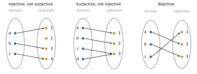
Surjectivity depends on the codomain you declare. \(x \mapsto x^2\) is not surjective onto \(\mathbb{R}\) (−1 is never hit) but is surjective onto \(\lbrack 0, \infty)\). Injectivity depends on the domain: \(x^2\) is not injective on \(\mathbb{R}\) but is on \(\lbrack 0, \infty)\). So \(x \mapsto x^2\) as a function \(\lbrack 0, \infty) \to \lbrack 0, \infty)\) is a bijection, and its inverse is the square root, matching what we found earlier.
Worked example. Classify, with reasons:
-
\(f : \mathbb{Z} \to \mathbb{Z},\ f(n) = 2n\). Injective: \(2n_1 = 2n_2 \Rightarrow n_1 = n_2\). Not surjective: 3 is not twice any integer. Not bijective.
-
\(g : \mathbb{R} \to \mathbb{R},\ g(x) = 2x\). Injective as before. Surjective: given any \(y\), \(x = y/2\) works. Bijective, with inverse \(y \mapsto y/2\). The same formula changed its classification because the sets changed.
-
\(h : \{0, 1, \ldots, 19\} \to \{0, 1, 2, 3, 4\},\ h(n) = n \bmod 5\). Surjective (0–4 are each hit, four times). Not injective (0 and 5 collide).
def is_injective(f, domain):
    seen = {}
    for x in domain:
        y = f(x)
        if y in seen:
            return False, (seen[y], x)    # two inputs, one output
        seen[y] = x
    return True, None

def is_surjective(f, domain, codomain):
    missed = set(codomain) - {f(x) for x in domain}
    return not missed, missed

D = range(-3, 4)
print(is_injective(lambda x: x ** 2, D))
print(is_injective(lambda x: 2 * x + 1, D))
print(is_surjective(lambda x: x % 5, range(20), range(5)))
print(is_surjective(lambda x: 2 * x, range(5), range(10)))
(False, (-1, 1))
(True, None)
(True, set())
(False, {1, 3, 5, 7, 9})
On a finite domain these checks are complete proofs: the program examines every input. The injectivity check is the same algorithm as "detect duplicate values with a dictionary".
|
How big is infinity?
Georg Cantor (1870s) defined two sets to have the same size when there is a bijection between them. Surprising consequences follow. The even numbers are "as many" as all natural numbers (pair \(n \leftrightarrow 2n\)), even though they are a proper subset. The rationals can be listed in a single sequence, so they too match the naturals. But the real numbers cannot: Cantor’s diagonal argument shows that any list of reals misses one. So there are different sizes of infinity, and the same diagonal argument, reused by Turing in 1936, shows that some problems (like deciding whether an arbitrary program halts) cannot be solved by any program. |
|
Collision finder
Type keys into a hash table with an adjustable number of buckets and a choice of hash function (length of string, sum of character codes, CRC32). Watch the buckets fill, count collisions, and compare against the "birthday" prediction that collisions appear after roughly \(\sqrt{n}\) keys in \(n\) buckets (Chapter 29). Then switch the codomain to as many buckets as keys and try to find a hash that is a bijection. |
11.12. Interactive tools
Browser tools on the companion website that go with this chapter. Each example link in the chapter opens one of them with that example already set up.
11.13. Exercises
-
(Recognition) Which of these are functions of \(x\)? (a) The relation \(\{(1, 2), (2, 3), (3, 2)\}\). (b) The relation \(\{(1, 2), (1, 3), (2, 4)\}\). (c) \(y^2 = x\). (d) \(y = x^3 - x\).
-
(Recognition) For \(f : \mathbb{R} \to \mathbb{R},\ f(x) = x^2 + 1\), state the domain, codomain and range.
-
(Application) Let \(f(x) = 3x^2 - x\). Find \(f(-2)\) and simplify \(f(x + h) - f(x)\).
-
(Application) Find the natural domain of (a) \(\dfrac{x + 1}{x^2 - 5x + 6}\) and (b) \(\sqrt{6 - 2x}\).
-
(Application) Describe the transformation from \(y = \sqrt{x}\) to \(y = 3\sqrt{x + 4} - 2\), and give the image of the point \((9, 3)\).
-
(Application) Let \(f(x) = 2x - 1\) and \(g(x) = x^2\). Find \((f \circ g)(x)\), \((g \circ f)(x)\) and \((f \circ f)(x)\).
-
(Application) Find the inverse of \(f(x) = \dfrac{x}{x + 1}\) and state its domain.
-
(Application) Classify as even, odd or neither: (a) \(x^5 - 2x^3\), (b) \(x^2 + \lvert x \rvert\), (c) \(x^3 + 1\).
-
(Application) Find the holes, vertical asymptotes and horizontal asymptote of \(R(x) = \dfrac{3x^2 - 3x}{x^2 - 1}\).
-
(Problem solving) A phone plan costs $20 per month including 5 GB of data, plus $10 per extra GB or part thereof. Write the monthly cost \(C(d)\) for data use \(d\) GB and find \(C(7.2)\).
-
(Problem solving) For \(f : \{0, 1, \ldots, 9\} \to \{0, 1, \ldots, 9\},\ f(n) = 3n \bmod 10\), decide whether \(f\) is bijective and, if so, find \(f^{-1}\). What changes if \(3\) is replaced by \(4\)?
-
(Problem solving) Explain why
random.random()is not a mathematical function, and describe how a library could provide a pure random-number generator.
Answers
-
(a) Function: each first coordinate appears once (2 is hit twice, which is allowed). (b) Not a function: input 1 has two outputs. (c) Not a function of \(x\): \(x = 4\) gives \(y = \pm 2\) (it fails the vertical line test). (d) Function.
-
Domain \(\mathbb{R}\), codomain \(\mathbb{R}\), range \(\lbrack 1, \infty)\) (since \(x^2 \ge 0\), \(x^2 + 1 \ge 1\), and every value \(\ge 1\) is reached at \(x = \sqrt{y - 1}\)).
-
\(f(-2) = 3(4) + 2 = 14\). \(f(x + h) = 3(x^2 + 2xh + h^2) - x - h = 3x^2 + 6xh + 3h^2 - x - h\), so \(f(x + h) - f(x) = 6xh + 3h^2 - h\). (Dividing by \(h\) gives \(6x + 3h - 1\); this difference quotient reappears in Chapter 17.)
-
(a) \(x^2 - 5x + 6 = (x - 2)(x - 3)\), so domain \(\mathbb{R} \setminus \{2, 3\}\). (b) \(6 - 2x \ge 0 \iff x \le 3\): domain \((-\infty, 3]\).
-
\(a = 3, b = 1, h = -4, k = -2\): shift left 4, stretch vertically by 3, shift down 2. \((9, 3) \mapsto (9 - 4,\ 3 \cdot 3 - 2) = (5, 7)\). Check: \(3\sqrt{5 + 4} - 2 = 9 - 2 = 7\).
-
\((f \circ g)(x) = 2x^2 - 1\); \((g \circ f)(x) = (2x - 1)^2 = 4x^2 - 4x + 1\); \((f \circ f)(x) = 2(2x - 1) - 1 = 4x - 3\).
-
\(y = x/(x + 1) \Rightarrow y(x + 1) = x \Rightarrow xy + y = x \Rightarrow y = x - xy = x(1 - y) \Rightarrow x = y/(1 - y)\). So \(f^{-1}(x) = \dfrac{x}{1 - x}\), domain \(x \ne 1\) (1 is the horizontal asymptote of \(f\), never reached). Check: \(f(1) = 1/2\), \(f^{-1}(1/2) = (1/2)/(1/2) = 1\).
-
(a) Odd: \((-x)^5 - 2(-x)^3 = -x^5 + 2x^3 = -(x^5 - 2x^3)\). (b) Even: \((-x)^2 + \lvert -x \rvert = x^2 + \lvert x \rvert\). (c) Neither: \(f(1) = 2\), \(f(-1) = 0\), which is neither \(2\) nor \(-2\).
-
\(R(x) = \dfrac{3x(x - 1)}{(x - 1)(x + 1)}\). Common factor \(x - 1\): hole at \(x = 1\), height \(3(1)/(1 + 1) = 3/2\), so the hole is at \((1, 3/2)\). Remaining denominator zero: vertical asymptote \(x = -1\). Equal degrees, leading coefficients 3 and 1: horizontal asymptote \(y = 3\).
-
\(C(d) = 20\) for \(0 \le d \le 5\); \(C(d) = 20 + 10\lceil d - 5 \rceil\) for \(d > 5\). (The single formula \(20 + 10\max(0, \lceil d - 5 \rceil)\) also works.) \(C(7.2) = 20 + 10\lceil 2.2 \rceil = 20 + 30 = 50\) dollars.
-
Outputs for \(n = 0, \ldots, 9\): 0, 3, 6, 9, 2, 5, 8, 1, 4, 7, all different and covering 0–9, so \(f\) is a bijection. Reading the table backwards, \(f^{-1}(m) = 7m \bmod 10\) (because \(3 \times 7 = 21 \equiv 1 \pmod{10}\); check \(f^{-1}(3) = 21 \bmod 10 = 1\)). With 4: outputs 0, 4, 8, 2, 6, 0, … only even numbers, so neither injective nor surjective. The difference is that 3 shares no factor with 10 while 4 does (Chapter 23).
-
Calling it twice with the same (empty) input gives different outputs, so it depends on a hidden input: the generator’s internal state, which each call also changes (a side effect). A pure design passes the state explicitly:
next_value, new_state = step(state). NumPy’sGeneratorobjects and JAX’s explicit random keys follow this idea.
11.14. Mastery check
-
State the definition of a function in one sentence, and explain why \(x^2 + y^2 = 25\) does not define \(y\) as a function of \(x\).
-
Find the natural domain of \(f(x) = \dfrac{\sqrt{x + 2}}{x^2 - 9}\) in interval notation.
-
Sketch \(g(x) = -\lvert x - 1 \rvert + 3\) by transforming \(\lvert x \rvert\); give the vertex and the \(x\)-intercepts.
-
Write \(h(x) = \sqrt{5 - x^3}\) as a composition \(f \circ g\) of two simpler functions, and find its domain.
-
Find the inverse of \(f(x) = \dfrac{4x - 1}{3}\) and verify it with one number.
-
Is \(f(x) = x^3 - 4x\) even, odd or neither? Prove it.
-
Give the asymptotes of \(R(x) = \dfrac{x + 5}{2x - 4}\).
-
For \(f : \{a, b, c, d\} \to \{1, 2, 3\}\), explain why \(f\) cannot be injective, and say what that implies for hash functions.
Decision rule: All correct without hesitation → move on to Chapter 12. Stuck on 1–2 → reread the relevant section (Section 11.2 for 2, Section 11.5 for 3, Section 11.7 for 5). Stuck on more → work the chapter exercises first.
Mastery check answers
-
A function from \(A\) to \(B\) assigns to each element of \(A\) exactly one element of \(B\). For \(x = 3\), both \(y = 4\) and \(y = -4\) satisfy the equation, so \(x = 3\) would have two outputs (the circle fails the vertical line test).
-
Root: \(x + 2 \ge 0 \iff x \ge -2\). Denominator: \(x^2 - 9 \ne 0 \iff x \ne \pm 3\); \(-3\) is already excluded. Domain: \(\lbrack -2, 3) \cup (3, \infty)\).
-
\(a = -1, h = 1, k = 3\): the V flipped upside down, corner (vertex) at \((1, 3)\). \(x\)-intercepts: \(\lvert x - 1 \rvert = 3 \iff x - 1 = \pm 3 \iff x = 4\) or \(x = -2\).
-
Inner \(g(x) = 5 - x^3\), outer \(f(u) = \sqrt{u}\). Domain: \(5 - x^3 \ge 0 \iff x^3 \le 5 \iff x \le \sqrt[3]{5}\), i.e. \((-\infty, \sqrt[3]{5}]\) (cubing is increasing, so the inequality direction is preserved).
-
\(y = (4x - 1)/3 \Rightarrow 3y = 4x - 1 \Rightarrow 3y + 1 = 4x \Rightarrow x = (3y + 1)/4\). So \(f^{-1}(x) = (3x + 1)/4\). Check: \(f(1) = 1\), \(f^{-1}(1) = 1\); better, \(f(4) = 5\), \(f^{-1}(5) = 16/4 = 4\).
-
Odd: \(f(-x) = (-x)^3 - 4(-x) = -x^3 + 4x = -(x^3 - 4x) = -f(x)\) for every \(x\).
-
Vertical: \(2x - 4 = 0 \iff x = 2\) (numerator \(x + 5\) is not zero there, so no hole). Horizontal: equal degrees, leading coefficients 1 and 2, so \(y = 1/2\).
-
Four inputs and three outputs: by the pigeonhole principle two inputs must share an output. Any hash function from a larger set of keys to a smaller set of buckets must have collisions; good hashing makes them rare and well spread, never impossible.