Chapter 7. Polynomials and Factoring

Volume 1: Foundations to Precalculus · Part II: Algebra

Chapter map: polynomials are the expressions you get when you are allowed to add, subtract and multiply, but never divide by the variable. They are the workhorse of algebra: they model areas, volumes, profits and trajectories; they are what computers evaluate when they approximate sine or exp; and they hide inside hash functions and network checksums. This chapter restores the vocabulary, the arithmetic, and the single most useful skill in elementary algebra, factoring, and treats each procedure as the algorithm it really is.

Where this chapter sits

You need: the rules of arithmetic and the distributive law from Chapter 1; fraction arithmetic from Chapter 2; exponent laws from Chapter 3; simplifying and expanding expressions from Chapter 4; and solving linear equations from Chapter 5.

This chapter unlocks: Chapter 8 (factoring is the first method for solving quadratics), Chapter 11 (polynomial functions are the first big family), Chapter 15 (every polynomial has a full set of complex roots), Chapter 17 (polynomials are the easiest functions to differentiate), Chapter 23 (polynomial arithmetic mirrors integer arithmetic), and Chapter 32 (Horner’s method, interpolation).

7.1. What a polynomial is

7.1.1. The problem

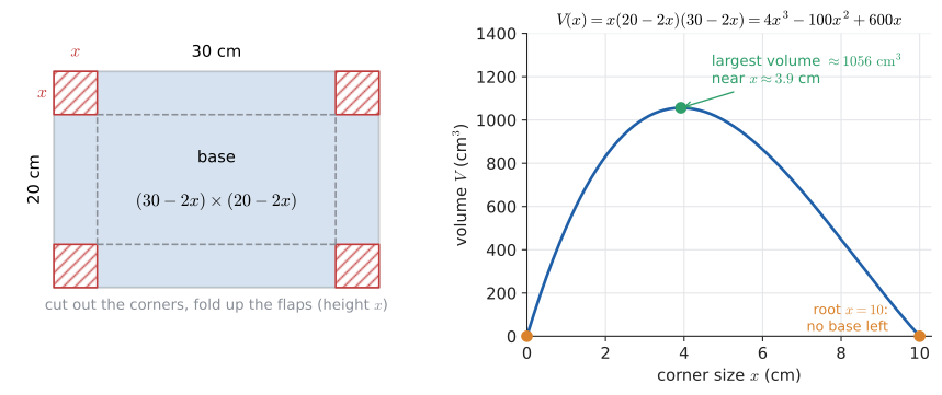
You have a 20 cm by 30 cm sheet of card. You cut an $x$ by $x$ square out of each corner and fold up the flaps to make an open box. How big should $x$ be to make the box hold as much as possible?

Write down the volume. The base is $(30 - 2x)$ long and $(20 - 2x)$ wide, and the box is $x$ tall, so

\[V(x) = x(20 - 2x)(30 - 2x).\]

That is a perfectly good formula, but before you can do much with it (graph it, find where it is zero, find its maximum) you need to know what kind of object it is. Multiplied out, it becomes $V(x) = 4x^3 - 100x^2 + 600x$. That is a polynomial, and the whole of this chapter is about how to read, combine, take apart and evaluate expressions like it. (The maximum itself needs calculus; we return to this box in Chapter 18.)

Left, a 30 by 20 rectangle with x by x squares hatched at each corner and dashed fold lines around the base. Right, the graph of V of x equals x times 20 minus 2x times 30 minus 2x for x from 0 to 10, rising from 0 to a peak of about 1056 cubic centimetres near x equals 3.9 and falling back to 0 at x equals 10

Figure 45. The open-box problem. Cutting $x$-by-$x$ corners from a 30 cm by 20 cm card leaves a base $(30 - 2x)$ by $(20 - 2x)$; the volume is a cubic in $x$. Its roots $x = 0$ and $x = 10$ are the two "no box" extremes, and the largest volume lies between them.

7.1.2. Intuition

A polynomial is anything you can build from a variable and some numbers using only addition, subtraction and multiplication. Because multiplication by $x$ repeated $k$ times gives $x^k$, every polynomial can be rearranged into a sum of pieces of the form number times a whole-number power of $x$:

\[4x^3 - 100x^2 + 600x + 0 .\]

Think of a polynomial as a list of numbers (the coefficients) attached to the slots $x^0, x^1, x^2, \ldots$. As a programmer you might store $4x^3 - 100x^2 + 600x$ as the array [4, -100, 600, 0]. That view, a polynomial is its coefficient list, turns out to be the key to almost every algorithm in this chapter.

What is not a polynomial? Anything with the variable in a denominator ($1/x$), under a root ($\sqrt{x}$), in an exponent ($2^x$), or inside a function like $\sin x$. Those have negative, fractional, or non-constant exponents, or no exponent form at all.

7.1.3. Vocabulary and notation

Term

A term is one of the pieces being added in an expression. In $7x^2 - 3x + 4$ the terms are $7x^2$, $-3x$ and $4$. The sign belongs to the term: the middle term is $-3x$, not $3x$.

Coefficient

A coefficient is the number multiplying a power of the variable. In $7x^2 - 3x + 4$, $7$ is the coefficient of $x^2$ and $-3$ is the coefficient of $x$. A missing power has coefficient $0$; a bare $x^2$ has coefficient $1$.

Constant term

The constant term is the term with no variable, i.e. the coefficient of $x^0$. In $7x^2 - 3x + 4$ it is $4$. It is the value of the polynomial at $x = 0$.

Polynomial

A polynomial in $x$ is an expression of the form

\[a_n x^n + a_{n-1} x^{n-1} + \cdots + a_1 x + a_0,\]

where $n$ is a non-negative whole number and the $a_k$ are constants (the coefficients). From Greek poly (many) plus Latin nomen (name, term): "many terms".

Degree

The degree of a polynomial is the highest power of the variable that appears with a non-zero coefficient. $4x^3 - 100x^2 + 600x$ has degree 3. A non-zero constant such as $5$ has degree 0. Names: degree 1 linear, 2 quadratic, 3 cubic, 4 quartic, 5 quintic.

Leading term and leading coefficient

The leading term is the term of highest degree; its coefficient is the leading coefficient. In $-2x^5 + x^2 - 9$ the leading term is $-2x^5$ and the leading coefficient is $-2$. A polynomial whose leading coefficient is $1$ is called monic.

Standard form

A polynomial is in standard form when like terms are combined and the terms are written in decreasing order of degree: $3x^4 - x^2 + 5x - 8$, not $5x - 8 + 3x^4 - x^2$.

Monomial, binomial, trinomial

Polynomials are also named by their number of terms (after combining like terms): a monomial has one term ($-6x^3$), a binomial two ($x^2 - 9$), a trinomial three ($x^2 + 5x + 6$). Beyond three we just say "polynomial".

Like terms

Like terms have the same variable raised to the same power: $3x^2$ and $-5x^2$ are like terms; $3x^2$ and $3x$ are not. Only like terms can be combined: $3x^2 - 5x^2 = -2x^2$.

Reading the notation. The general form $a_n x^n + a_{n-1}x^{n-1} + \cdots + a_1 x + a_0$ packs in a lot. The subscript on $a_k$ is just a label, matching the power of $x$ the coefficient sits in front of: $a_3$ is the coefficient of $x^3$. The dots $\cdots$ mean "carry on the pattern". So for $4x^3 - 100x^2 + 600x$ we have $n = 3$, $a_3 = 4$, $a_2 = -100$, $a_1 = 600$, $a_0 = 0$.

You will also see the same thing written with the summation sign $\Sigma$ (capital Greek sigma, for "sum"):

\[p(x) = \sum_{k=0}^{n} a_k x^k .\]

Read this as: "let $k$ run through the whole numbers from the value under the sigma ($0$) to the value on top ($n$); for each one write down $a_k x^k$; add them all up." It is exactly a for k in range(0, n + 1) loop accumulating a sum. The notation $p(x)$ names the polynomial and says what its variable is, so $p(2)$ means "substitute $2$ for $x$".

7.1.4. Visualization: what the degree tells you about the graph

Far from the origin, the leading term dominates every other term: when $x = 1000$, $4x^3$ is four billion while $-100x^2$ is a mere hundred million. So the ends of a polynomial’s graph are controlled by the leading term alone: its degree (even or odd) and the sign of its coefficient.

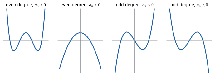
Four small graphs: even degree with positive leading coefficient rises at both ends; even degree negative falls at both ends; odd degree positive falls left and rises right; odd degree negative rises left and falls right

Figure 46. End behaviour is set by the leading term alone

Even degree: both ends go the same way (up if $a_n > 0$, down if $a_n < 0$). Odd degree: the ends go opposite ways. A polynomial of degree $n$ can turn around at most $n - 1$ times, and crosses the $x$-axis at most $n$ times; we will see why in Section 7.6.

7.1.5. Worked example: putting a polynomial in standard form

Write the box volume $V(x) = x(20 - 2x)(30 - 2x)$ in standard form, and state its degree, leading coefficient and constant term.

\[\begin{aligned} (20 - 2x)(30 - 2x) &= 20\cdot 30 + 20\cdot(-2x) + (-2x)\cdot 30 + (-2x)(-2x) && \text{(distribute)}\\ &= 600 - 40x - 60x + 4x^2 &&\\ &= 4x^2 - 100x + 600 && \text{(combine like terms, order by degree)}\\ V(x) &= x\,(4x^2 - 100x + 600) &&\\ &= 4x^3 - 100x^2 + 600x && \text{(distribute the } x\text{)} \end{aligned}\]

Degree 3 (a cubic), leading coefficient $4$, constant term $0$. The zero constant term tells you $V(0) = 0$: no cut, no box. That is a sanity check worth doing whenever you build a model.

7.1.6. Where you’d use this

Polynomials are the formulas you get from adding up products, so they turn up whenever quantities compound, accumulate or are approximated.

Saving. Put $1000 into an account at the start of each year for three years at interest rate $r$. Writing $g = 1 + r$ for the yearly growth factor, the balance at the end of year 3 is $1000g^3 + 1000g^2 + 1000g$, a cubic in $g$. At 5% ($g = 1.05$) that is $1157.625 + 1102.50 + 1050.00 = 3310.125$, or \$3310.13 to the nearest cent. Pension and loan calculators evaluate polynomials like this, and solving one for $g$ (the "interest rate that makes the numbers work") is root-finding.
Mechanics and engineering. Displacement under constant acceleration, $s = ut + \tfrac12 at^2$, is a polynomial in $t$. The sag of a cantilever beam under a uniform load is a quartic in the distance along the beam. Temperature sensors (thermocouples) are calibrated with published polynomials that turn a voltage into a temperature.
Computing. Hardware has no "sine" instruction to lean on: math libraries reduce the angle to a small range and then evaluate a carefully chosen polynomial. Even three terms do well near 0: $x - \frac{x^3}{6} + \frac{x^5}{120}$ at $x = 0.5$ gives $0.4794271$, against the true $\sin 0.5 = 0.4794255$. The curves in every font and vector drawing are cubic (or quadratic) polynomial pieces. Evaluating polynomials fast and accurately is the subject of Horner’s method (Section 7.8).

Why "polynomial" and not "multinomial"?

"Polynomial" is a hybrid of Greek poly and Latin nomen, the kind of mongrel word purists hated. It was coined by analogy with "binomial", which goes back to the sixteenth century. Mathematicians before Descartes (1637) wrote polynomials in words or idiosyncratic abbreviations; Descartes’s convention of letters near the end of the alphabet ($x, y, z$) for unknowns and letters near the start ($a, b, c$) for known quantities is the one we still use.

US curriculum

Polynomial vocabulary (term, degree, monomial/binomial/trinomial, standard form) and adding/subtracting/multiplying polynomials appear in Algebra I (grades 8–9). End behaviour and polynomial functions of higher degree are Algebra II topics (grades 10–11).

7.2. Adding, subtracting and multiplying polynomials

7.2.1. The problem

A company’s revenue from selling $q$ units is $R(q) = 40q - 0.01q^2$ and its cost is $C(q) = 5000 + 12q$. What is its profit? Profit is revenue minus cost, so you need to subtract one polynomial from another. Later, if the number of units sold is itself a polynomial in time, you will need to multiply and substitute. Polynomial arithmetic is how you combine models.

7.2.2. Intuition and why it works

Every rule here is a consequence of the ordinary laws of arithmetic you met in Chapter 1:

commutativity ($a + b = b + a$, $ab = ba$) and associativity let you reorder and regroup terms;
the distributive law $a(b + c) = ab + ac$ lets you combine like terms ($3x^2 + 5x^2 = (3 + 5)x^2$) and multiply out brackets;
the exponent law $x^m \cdot x^n = x^{m+n}$ from Chapter 3 tells you what happens to powers when terms multiply.

Adding polynomials is adding coefficient lists slot by slot. Subtracting is the same after negating every coefficient of the second polynomial. Multiplying is "every term of the first times every term of the second, then collect".

7.2.3. Worked example: adding and subtracting

\[\begin{aligned} (3x^2 - 5x + 2) + (x^3 - 2x^2 + 7) &= x^3 + (3 - 2)x^2 + (-5)x + (2 + 7) &&\text{(group like terms)}\\ &= x^3 + x^2 - 5x + 9. \end{aligned}\]

For subtraction, distribute the minus sign over the whole second bracket first:

\[\begin{aligned} (4x^3 - 2x + 1) - (x^3 + 3x^2 - 2x - 6) &= 4x^3 - 2x + 1 - x^3 - 3x^2 + 2x + 6 &&\text{(negate every term)}\\ &= (4 - 1)x^3 - 3x^2 + (-2 + 2)x + (1 + 6) &&\text{(group)}\\ &= 3x^3 - 3x^2 + 7. \end{aligned}\]

And the profit from the problem: $P(q) = R(q) - C(q) = 40q - 0.01q^2 - 5000 - 12q = -0.01q^2 + 28q - 5000$, a quadratic. (Chapter Chapter 8 finds its break-even points and its maximum.)

Distributing the minus sign

The single most common slip in polynomial arithmetic is writing $(4x^3 - 2x + 1) - (x^3 + 3x^2 - 2x - 6)$ as $4x^3 - 2x + 1 - x^3 + 3x^2 - 2x - 6$, negating only the first term. The minus sign multiplies the whole bracket, so every sign inside flips. If in doubt, rewrite the subtraction as adding $(-1)\times(\ldots)$.

7.2.4. Multiplication and the area model

To multiply two polynomials, multiply every term of the first by every term of the second and add the results. Why? Apply the distributive law twice:

\[\begin{aligned} (x + 3)(x + 2) &= x(x + 2) + 3(x + 2) &&\text{(distribute over the first bracket)}\\ &= x^2 + 2x + 3x + 6 &&\text{(distribute again)}\\ &= x^2 + 5x + 6. &&\text{(combine like terms)} \end{aligned}\]

The picture makes this obvious. A rectangle $(x + 3)$ wide and $(x + 2)$ tall has area $(x + 3)(x + 2)$. Cut it along the joins and it falls into four pieces, one per pair of terms:

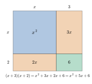
A rectangle with width x plus 3 and height x plus 2, divided into four cells with areas x squared, 3x, 2x and 6

Figure 47. The area model: each cell is one term-by-term product

For longer polynomials the same idea becomes a grid: write the terms of one polynomial across the top, the other down the side, fill each cell with the product, then add along diagonals of equal degree. It is literally the long-multiplication algorithm from primary school, without the carries.

FOIL

FOIL (First, Outer, Inner, Last) is a US mnemonic for multiplying two binomials: $(a + b)(c + d) = ac + ad + bc + bd$. It is not a separate rule, just the distributive law (the four cells of a 2-by-2 area model) with a fixed order. It does not extend to longer polynomials; the grid does.

Example 39. Procedure — Multiplying polynomials

Input: polynomials $p(x)$ with terms $p_1, \ldots, p_m$ and $q(x)$ with terms $q_1, \ldots, q_k$.

Steps:

For every pair $(p_i, q_j)$, multiply coefficients and add exponents: $ax^r \cdot bx^s = ab\,x^{r+s}$.
Collect the $mk$ products.
Combine like terms and write the result in standard form.
Check: the degree of the product must be $\deg p + \deg q$, and the leading coefficient must be the product of the two leading coefficients.

Output: $p(x)\,q(x)$ in standard form.

7.2.5. Worked example: a binomial times a trinomial

Expand $(2x - 3)(x^2 + 4x - 5)$.

\[\begin{aligned} (2x - 3)(x^2 + 4x - 5) &= 2x\cdot x^2 + 2x\cdot 4x + 2x\cdot(-5) + (-3)\cdot x^2 + (-3)\cdot 4x + (-3)(-5) &&\text{(six products)}\\ &= 2x^3 + 8x^2 - 10x - 3x^2 - 12x + 15 &&\\ &= 2x^3 + (8 - 3)x^2 + (-10 - 12)x + 15 &&\text{(group like terms)}\\ &= 2x^3 + 5x^2 - 22x + 15. \end{aligned}\]

Check: degree $1 + 2 = 3$ ✓; leading coefficient $2 \cdot 1 = 2$ ✓; constant term $(-3)(-5) = 15$ ✓. A fourth check that catches almost everything: substitute an easy value. At $x = 1$ the left side is $(-1)(1 + 4 - 5) = 0$ and the right side is $2 + 5 - 22 + 15 = 0$ ✓.

7.2.6. Alternative approaches and method selection

Distribute term by term (as above) is the default for anything up to about three terms by three.
Grid is better for longer polynomials, because it is easy to see you have not missed a product.
Special-product patterns (next section) are faster when they apply: $(x - 7)(x + 7)$ should be written down as $x^2 - 49$ without any work at all.
Coefficient-list convolution (below) is what a computer does.

Computer-science connection: polynomial multiplication is convolution

Store a polynomial as its coefficient list, lowest power first or highest first, as long as you are consistent. Then the coefficient of $x^k$ in the product $p \cdot q$ is

\[c_k = \sum_{i + j = k} a_i\, b_j ,\]

"add up every product of a coefficient from $p$ and one from $q$ whose powers add to $k$". That operation on two lists has a name: convolution. It is the same operation as blurring an image with a kernel, computing a moving average, or combining two probability distributions of independent dice (Chapter 29).

def poly_mul(a, b):
    """Multiply polynomials given as coefficient lists (highest power first)."""
    out = [0] * (len(a) + len(b) - 1)
    for i, ai in enumerate(a):
        for j, bj in enumerate(b):
            out[i + j] += ai * bj
    return out

print(poly_mul([2, -3], [1, 4, -5]))      # (2x - 3)(x^2 + 4x - 5)

import numpy as np
print(np.convolve([2, -3], [1, 4, -5]))   # NumPy calls it convolve

[2, 5, -22, 15]
[  2   5 -22  15]

The double loop costs $O(nm)$ multiplications. For very long polynomials (multiplying million-digit integers, which are polynomials in the base 10 or $2^{64}$) the Fast Fourier Transform does it in $O(n \log n)$; see Chapter 32.

Grid multiplier

Type two polynomials; the lab draws the area-model grid with each cell sized by its term (for positive values of $x$) and colours cells of equal degree the same. Slide $x$ and watch the total area equal the product of the side lengths.

7.3. Special products

7.3.1. The problem

Some products come up so often that recognising them on sight saves enormous time, and, more importantly, lets you run them backwards when factoring. Can you compute $47 \times 53$ in your head? You can if you notice that $47 \times 53 = (50 - 3)(50 + 3)$.

7.3.2. The four patterns, and why they work

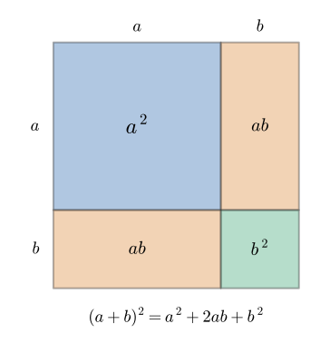
Perfect square. Expand by the distributive law:

\[\begin{aligned} (a + b)^2 &= (a + b)(a + b) = a^2 + ab + ba + b^2 = a^2 + 2ab + b^2,\\ (a - b)^2 &= a^2 - 2ab + b^2. \end{aligned}\]

The picture: a square of side $a + b$ is made of an $a^2$ square, a $b^2$ square, and two $a \times b$ rectangles. The two rectangles are why the middle term is $2ab$.

A square of side a plus b split into a squared, two rectangles of area ab, and b squared

Figure 48. The perfect-square identity as an area

Difference of squares.

\[(a + b)(a - b) = a^2 - ab + ba - b^2 = a^2 - b^2 .\]

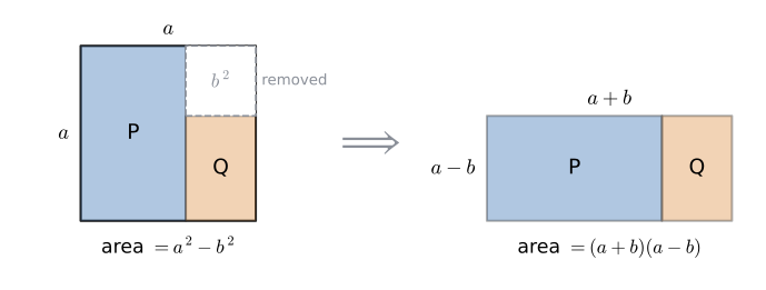
The middle terms cancel. Geometrically: take an $a \times a$ square and remove a $b \times b$ corner. The L-shaped remainder can be cut into two rectangles and rearranged into a single rectangle $(a + b)$ long and $(a - b)$ high.

On the left, an a by a square with a b by b corner removed, cut into pieces P and Q; on the right, the same pieces rearranged into a rectangle of width a plus b and height a minus b

Figure 49. Difference of squares: cut the L-shape and re-assemble it

Sum and difference of cubes.

\[\begin{aligned} a^3 + b^3 &= (a + b)(a^2 - ab + b^2),\\ a^3 - b^3 &= (a - b)(a^2 + ab + b^2). \end{aligned}\]

Verify the second by multiplying out, and watch four of the six terms cancel in pairs:

\[\begin{aligned} (a - b)(a^2 + ab + b^2) &= a^3 + a^2 b + ab^2 - a^2 b - ab^2 - b^3 &&\text{(six products)}\\ &= a^3 - b^3. &&\text{(}{\pm a^2 b}\text{ and }{\pm ab^2}\text{ cancel)} \end{aligned}\]

The first follows by replacing $b$ with $-b$. A memory aid for the signs is "SOAP": the binomial has the Same sign as the original, the next sign is the Opposite, and the last is Always Positive.

Special products

\[\begin{aligned} (a \pm b)^2 &= a^2 \pm 2ab + b^2 \\ (a + b)(a - b) &= a^2 - b^2 \\ a^3 \pm b^3 &= (a \pm b)(a^2 \mp ab + b^2) \end{aligned}\]

The $\pm$ ("plus or minus") and $\mp$ ("minus or plus") signs mean: read all top signs together, or all bottom signs together.

7.3.3. Worked examples

$47 \times 53 = (50 - 3)(50 + 3) = 50^2 - 3^2 = 2500 - 9 = 2491.$
$99^2 = (100 - 1)^2 = 10000 - 200 + 1 = 9801.$
$(3x - 5)^2 = (3x)^2 - 2(3x)(5) + 5^2 = 9x^2 - 30x + 25.$
$(2x + 7y)(2x - 7y) = (2x)^2 - (7y)^2 = 4x^2 - 49y^2.$
$(x + 2)(x^2 - 2x + 4) = x^3 + 2^3 = x^3 + 8.$

The freshman’s dream

$(a + b)^2 \neq a^2 + b^2$. Test it: $(3 + 4)^2 = 49$ but $3^2 + 4^2 = 25$. The missing $24$ is the two rectangles $2ab$ in the picture. Squaring does not distribute over addition, and neither does taking square roots: $\sqrt{9 + 16} = 5 \neq 3 + 4$. The same error in a compiler would be an invalid optimisation.

Mental arithmetic with algebra

Before electronic calculators, surveyors and astronomers used tables of quarter-squares to multiply: since $(a + b)^2 - (a - b)^2 = 4ab$,

\[ab = \frac{(a + b)^2}{4} - \frac{(a - b)^2}{4},\]

so one table of $n^2/4$ plus two lookups and a subtraction replaces a multiplication. Some early analogue and digital multipliers worked the same way.

US curriculum

Special products (perfect squares, difference of squares) are Algebra I; sum and difference of cubes usually wait for Algebra II.

7.4. Factoring

7.4.1. The problem

Solve $x^3 - 2x^2 - 5x + 6 = 0$.

There is no "isolate $x$" move here: $x$ appears to three different powers. But suppose you knew that

\[x^3 - 2x^2 - 5x + 6 = (x + 2)(x - 1)(x - 3).\]

Then the problem collapses. A product of numbers is zero exactly when one of the numbers is zero, so the solutions are $x = -2$, $x = 1$ and $x = 3$. Factoring turns one hard equation into several easy ones.

Zero-product property

If $AB = 0$ then $A = 0$ or $B = 0$ (or both). This is why factoring solves equations. It works only with zero on the right: $AB = 6$ tells you nothing about $A$ or $B$ individually.

7.4.2. Intuition

Factoring is multiplication run backwards. Expanding $(x + 2)(x - 1)(x - 3)$ is mechanical; recovering the factors from $x^3 - 2x^2 - 5x + 6$ is a search problem, rather like factoring $391$ into $17 \times 23$ is harder than multiplying. For polynomials there is no single formula that always works, but there is a reliable decision procedure that handles almost everything you meet by hand.

Factor

A factor of an expression is something that divides it exactly, so that the expression equals the factor times something else. $(x - 3)$ is a factor of $x^2 - 9$ because $x^2 - 9 = (x - 3)(x + 3)$. To factor (British: to factorise) means to rewrite a sum as a product.

Greatest common factor (GCF)

The greatest common factor of several terms is the largest expression dividing all of them. For $6x^3 - 9x^2$ it is $3x^2$, so $6x^3 - 9x^2 = 3x^2(2x - 3)$. Take the GCF of the coefficients and the lowest power of each variable that appears in every term.

Irreducible (prime) polynomial

A polynomial is irreducible over a given number system if it cannot be written as a product of two polynomials of lower degree with coefficients in that system. $x^2 + 4$ is irreducible over the real numbers; $x^2 - 2$ is irreducible over the rationals but factors over the reals as $(x - \sqrt 2)(x + \sqrt 2)$. "Factor completely" means: keep going until every factor is irreducible (usually over the integers or rationals, unless stated).

7.4.3. The method: a decision procedure

Flowchart: pull out common factor; branch on number of terms to special patterns, trinomial method, or grouping; fall back to finding a root and dividing; repeat on each factor; check by multiplying

Figure 50. Factoring as a decision procedure

Example 40. Procedure — Factoring a polynomial completely

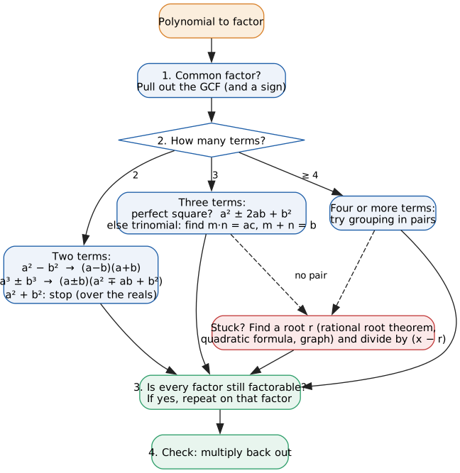
Input: a polynomial $p(x)$ with integer coefficients.

Steps:

Common factor. Pull out the GCF of all terms. If the leading coefficient is negative, pull out $-1$ too.
Count the terms of what remains.
1. Two terms: look for $a^2 - b^2$, $a^3 - b^3$, $a^3 + b^3$. (A sum of squares $a^2 + b^2$ does not factor over the reals.)
2. Three terms: look for a perfect square $a^2 \pm 2ab + b^2$; otherwise use the trinomial ($ac$) method below.
3. Four terms: try grouping into pairs.
Fallback: if nothing fits, find a root $r$ (rational root theorem, Section 7.7, or the quadratic formula for degree 2) and divide by $(x - r)$ (Section 7.5).
Recurse: apply the procedure again to every factor of degree 2 or more.
Check by multiplying back out (or substituting a test value).

Output: $p(x)$ as a product of irreducible factors.

7.4.4. The trinomial (ac) method

For a quadratic trinomial $ax^2 + bx + c$, you want to undo the area model: find the two middle cells. Their product must equal $ac$ (the product of the two corner cells, $ax^2$ and $c$, has coefficient $ac$), and their sum must be $b$.

Example 41. Procedure — Factoring $ax^2 + bx + c$ (the ac method)

Input: integers $a, b, c$ with $a \neq 0$.

Steps:

Compute $ac$.
Find integers $m, n$ with $mn = ac$ and $m + n = b$. (List the factor pairs of $ac$; signs: if $ac > 0$ both have the sign of $b$; if $ac < 0$ they have opposite signs.) If no pair exists, the trinomial does not factor over the integers: stop.
Split the middle term: $ax^2 + mx + nx + c$.
Group in pairs and pull out the common factor of each pair; a common binomial appears.
Pull out the common binomial.

Output: $(px + q)(rx + s)$, or "irreducible over the integers".

When $a = 1$ the method simplifies: $x^2 + bx + c = (x + m)(x + n)$ where $mn = c$ and $m + n = b$. For $x^2 + 5x + 6$: $2 \times 3 = 6$, $2 + 3 = 5$, so $(x + 2)(x + 3)$.

7.4.5. Worked example: the ac method

Factor $6x^2 + 7x - 3$.

$ac = 6 \times (-3) = -18$. Negative, so $m$ and $n$ have opposite signs.
Factor pairs of $-18$ and their sums: $(-1, 18)\to 17$, $(1, -18)\to -17$, $(-2, 9)\to 7$ ✓. So $m = 9$, $n = -2$.
Split and group:

\[\begin{aligned} 6x^2 + 7x - 3 &= 6x^2 + 9x - 2x - 3 &&\text{(split } 7x = 9x - 2x\text{)}\\ &= 3x(2x + 3) - 1(2x + 3) &&\text{(factor each pair)}\\ &= (2x + 3)(3x - 1). &&\text{(pull out } (2x+3)\text{)} \end{aligned}\]

Check: $(2x + 3)(3x - 1) = 6x^2 - 2x + 9x - 3 = 6x^2 + 7x - 3$ ✓.

7.4.6. Worked examples: running the whole procedure

(a) $2x^3 - 8x$.

\[\begin{aligned} 2x^3 - 8x &= 2x(x^2 - 4) &&\text{(GCF } 2x\text{)}\\ &= 2x(x - 2)(x + 2). &&\text{(difference of squares)} \end{aligned}\]

(b) $x^4 - 16$.

\[\begin{aligned} x^4 - 16 &= (x^2)^2 - 4^2 = (x^2 - 4)(x^2 + 4) &&\text{(difference of squares)}\\ &= (x - 2)(x + 2)(x^2 + 4). &&\text{(again; } x^2 + 4 \text{ is a sum of squares: stop)} \end{aligned}\]

(c) $x^3 + 2x^2 - 9x - 18$ (four terms: group).

\[\begin{aligned} x^3 + 2x^2 - 9x - 18 &= x^2(x + 2) - 9(x + 2) &&\text{(factor each pair)}\\ &= (x + 2)(x^2 - 9) &&\text{(common binomial)}\\ &= (x + 2)(x - 3)(x + 3). &&\text{(difference of squares)} \end{aligned}\]

(d) $3x^3 - 24$.

\[\begin{aligned} 3x^3 - 24 &= 3(x^3 - 8) &&\text{(GCF)}\\ &= 3(x - 2)(x^2 + 2x + 4). &&\text{(difference of cubes, } a = x,\ b = 2\text{)} \end{aligned}\]

The quadratic factor $x^2 + 2x + 4$ has $ac = 4$ with factor pairs summing to $4, 5, -4, -5$, never $2$; it is irreducible over the integers (in fact over the reals, as Chapter 8 will show via its discriminant, $4 - 16 < 0$).

(e) $4x^2 - 12x + 9$. Three terms; first and last are squares ($(2x)^2$ and $3^2$) and the middle is $-2(2x)(3)$. Perfect square: $(2x - 3)^2$.

7.4.7. Choosing a method

The order in the procedure is not arbitrary. Common factor first, because it shrinks everything else (try factoring $6x^2 + 42x + 72$ without first removing the $6$). Patterns next, because they are instant when they fit. The $ac$ method and grouping are systematic but slower. Root-finding plus division is the heavy machinery: it always works for a polynomial that has a rational root, but it is overkill for $x^2 - 9$.

Factoring traps

Stopping too early. $x^4 - 16 = (x^2 - 4)(x^2 + 4)$ is not finished; $x^2 - 4$ still factors.
Forgetting the GCF, then getting stuck in the $ac$ method with huge numbers.
Cancelling a variable instead of factoring it out. Dividing both sides of $x^3 = 4x$ by $x$ loses the solution $x = 0$. Instead write $x^3 - 4x = x(x - 2)(x + 2) = 0$.
Most polynomials do not factor nicely. $x^2 + x - 1$ has no integer factorisation. Textbook exercises are chosen to factor; real-world polynomials usually are not. That is why root formulas and numerical methods exist (Chapter 8, Chapter 32).

7.4.8. Where you’d use this

Factoring is how you solve "when does this polynomial equal zero?" by hand, via the zero-product property.

Dimensions from an area. A rectangular vegetable bed must have area 96 m² and be 4 m longer than it is wide. With width $x$: $x(x + 4) = 96$, so $x^2 + 4x - 96 = 0$, which factors as $(x + 12)(x - 8) = 0$. The width is 8 m (the root $-12$ is meaningless here), so the bed is 8 m by 12 m.
Projectiles. A ball kicked straight up at 20 m/s has height $h = 20t - 5t^2$ (taking $g \approx 10\ \text{m/s}^2$). Pulling out the common factor gives $h = 5t(4 - t)$, so it is at ground level at $t = 0$ and lands at $t = 4$ s. No formula needed: the factored form is the answer.
Computing. The Reed–Solomon codes that let a scratched CD play and a smudged QR code scan detect where errors are by finding the roots of an "error-locator" polynomial (over a finite field), which amounts to factoring it into linear pieces.

Factoring is a search problem

Factoring integer polynomials by hand is a bounded search: the $ac$ method enumerates factor pairs; the rational root theorem enumerates a finite candidate list. Computer-algebra systems use far cleverer algorithms (factoring modulo a prime, then "lifting"), and remarkably, factoring polynomials over the rationals can be done in polynomial time, while factoring large integers is believed to be hard, which is precisely what RSA encryption relies on (Chapter 23).

Factor explorer

Drag the two binomials $(px + q)$ and $(rx + s)$ by adjusting $p, q, r, s$; the lab shows the expanded trinomial and its area model. Then flip modes: given a trinomial, rearrange the tiles of an algebra-tile set into a rectangle, or discover that no rectangle exists.

7.5. Polynomial division

7.5.1. The problem

You know that $x = 1$ is a root of $x^3 - 2x^2 - 5x + 6$ (check: $1 - 2 - 5 + 6 = 0$). That should mean $(x - 1)$ is a factor. But what is the other factor? You need to divide $x^3 - 2x^2 - 5x + 6$ by $x - 1$. More generally, dividing polynomials is how you simplify rational expressions, find slant asymptotes (Chapter 11), and compute checksums.

7.5.2. Intuition: it is just long division

Recall long division of integers: to divide $7493$ by $23$, you ask "how many 23s fit into 74?", write 3, subtract $69$, bring down the next digit, and repeat. The output is a quotient and a remainder, and

\[7493 = 23 \times 325 + 18, \qquad 0 \le 18 < 23 .\]

Polynomial division is the same algorithm with "how many fit?" replaced by "what do I multiply the divisor’s leading term by to match the current leading term?" It is actually easier than integer division, because there are no carries and no guessing.

Dividend, divisor, quotient, remainder

In $p(x) \div d(x)$, $p$ is the dividend and $d$ the divisor. Division produces a quotient $q(x)$ and remainder $r(x)$ such that

\[p(x) = d(x)\,q(x) + r(x), \qquad \deg r < \deg d \text{ (or } r = 0\text{).}\]

If $r = 0$, $d$ divides $p$ exactly, and $d$ is a factor of $p$.

7.5.3. The method: long division

Example 42. Procedure — Polynomial long division

Input: dividend $p(x)$ and non-zero divisor $d(x)$, both in standard form. Insert a zero coefficient for every missing power in $p$.

Steps:

Divide the leading term of the current dividend by the leading term of $d$. Write the result as the next term of the quotient.
Multiply the whole divisor by that term.
Subtract the product from the current dividend. (The leading term cancels, by construction.)
If the degree of what remains is still $\ge \deg d$, it becomes the new current dividend: go to step 1.

Output: quotient $q(x)$ (the terms you wrote down) and remainder $r(x)$ (what is left).

Each pass removes the leading term, so the degree drops by at least one each time; the loop must terminate after at most $\deg p - \deg d + 1$ passes.

7.5.4. Worked example: long division

Divide $2x^3 + 3x^2 - 4x + 5$ by $x^2 + 2x - 1$.

Pass 1. Leading terms: $2x^3 \div x^2 = 2x$. Multiply: $2x(x^2 + 2x - 1) = 2x^3 + 4x^2 - 2x$. Subtract:

\[(2x^3 + 3x^2 - 4x + 5) - (2x^3 + 4x^2 - 2x) = -x^2 - 2x + 5 .\]

Pass 2. $-x^2 \div x^2 = -1$. Multiply: $-1\cdot(x^2 + 2x - 1) = -x^2 - 2x + 1$. Subtract:

\[(-x^2 - 2x + 5) - (-x^2 - 2x + 1) = 4 .\]

Degree 0 is less than 2, so stop. Quotient $2x - 1$, remainder $4$:

\[2x^3 + 3x^2 - 4x + 5 = (x^2 + 2x - 1)(2x - 1) + 4 .\]

Check: $(x^2 + 2x - 1)(2x - 1) = 2x^3 - x^2 + 4x^2 - 2x - 2x + 1 = 2x^3 + 3x^2 - 4x + 1$; add $4$ to get the dividend ✓.

In the traditional layout this looks like integer long division:

                 2x   -  1
            ________________________
x² + 2x - 1 ) 2x³ + 3x² - 4x + 5
              2x³ + 4x² - 2x
              ---------------
                  - x² - 2x + 5
                  - x² - 2x + 1
                  -------------
                              4

The algorithm, on coefficient lists:

def poly_divide(num, den):
    """Long division of polynomials (coefficient lists, highest power first).

    Returns (quotient, remainder) as coefficient lists.
    """
    num = list(num)
    q = []
    while len(num) >= len(den):
        factor = num[0] / den[0]
        q.append(factor)
        for i in range(len(den)):
            num[i] -= factor * den[i]
        num.pop(0)                       # leading term is now zero
    return q, num

print(poly_divide([2, 3, -4, 5], [1, 2, -1]))

([2.0, -1.0], [0.0, 4.0])

The remainder list [0.0, 4.0] means $0x + 4$.

7.5.5. Synthetic division: the fast path for $(x - r)$

When the divisor is the linear factor $x - r$, long division simplifies dramatically. Every pass multiplies the divisor by a single number and subtracts; tracking only the coefficients, the whole thing collapses into one row of "multiply by $r$, add the next coefficient".

Example 43. Procedure — Synthetic division by $(x - r)$

Input: coefficients $a_n, a_{n-1}, \ldots, a_0$ of $p(x)$ (with zeros for missing powers) and the number $r$. Note: for divisor $x + 3$, $r = -3$.

Steps:

Bring down $a_n$: set $b_{n-1} = a_n$.
For each subsequent coefficient: multiply the last value by $r$ and add the next coefficient.
The final value is the remainder; the earlier values are the quotient’s coefficients (one degree lower than $p$).

Output: quotient coefficients and remainder.

7.5.6. Worked example: synthetic division

Divide $x^3 - 2x^2 - 5x + 6$ by $x - 1$ (so $r = 1$):

 r = 1 |  1   -2   -5    6
       |       1   -1   -6
       +-------------------
          1   -1   -6  | 0

Step by step: bring down $1$. $1 \times 1 + (-2) = -1$. $-1 \times 1 + (-5) = -6$. $-6 \times 1 + 6 = 0$. Remainder $0$, quotient $x^2 - x - 6$. So

\[x^3 - 2x^2 - 5x + 6 = (x - 1)(x^2 - x - 6) = (x - 1)(x - 3)(x + 2),\]

finishing the problem we started with.

A second example with a missing term and a non-zero remainder: divide $2x^3 - 3x^2 + 5$ by $x - 2$. The coefficients are $2, -3, 0, 5$ (note the $0$ for the missing $x$ term).

 r = 2 |  2   -3    0    5
       |       4    2    4
       +-------------------
          2    1    2  | 9

Quotient $2x^2 + x + 2$, remainder $9$.

def synthetic_division(coeffs, r):
    """Divide a polynomial by (x - r).

    coeffs: highest power first. Returns (quotient_coeffs, remainder).
    """
    out = [coeffs[0]]
    for c in coeffs[1:]:
        out.append(out[-1] * r + c)
    return out[:-1], out[-1]

print(synthetic_division([1, -2, -5, 6], 1))
print(synthetic_division([2, -3, 0, 5], 2))

([1, -1, -6], 0)
([2, 1, 2], 9)

Missing terms and the sign of r

Leave a zero for every missing power. Dividing $2x^3 - 3x^2 + 5$ with coefficients [2, -3, 5] silently computes the wrong thing (it divides $2x^2 - 3x + 5$).
Dividing by $x + 3$ means $r = -3$, not $+3$.
Synthetic division as written only handles divisors $x - r$. For $2x - 1$, divide by $x - \tfrac12$ and then divide the quotient by $2$, or use long division.

Choosing a method. Linear divisor $x - r$: synthetic division, always. Anything else: long division.

US curriculum

Polynomial long division and synthetic division are Algebra II topics (grades 10–11), revisited in Precalculus for rational functions and asymptotes.

7.6. The remainder theorem, the factor theorem, and roots versus factors

7.6.1. The problem

In the last example, the remainder on dividing $2x^3 - 3x^2 + 5$ by $x - 2$ was $9$. Now evaluate the polynomial at $x = 2$: $2(8) - 3(4) + 5 = 16 - 12 + 5 = 9$. Coincidence?

7.6.2. Why it works

Divide any polynomial $p(x)$ by $x - r$. The remainder has degree less than 1, so it is a constant, call it $R$:

\[p(x) = (x - r)\,q(x) + R .\]

This identity holds for every $x$. Substitute $x = r$:

\[p(r) = (r - r)\,q(r) + R = 0 \cdot q(r) + R = R .\]

That is the whole proof. Two consequences, each worth a name:

Remainder theorem

The remainder when $p(x)$ is divided by $(x - r)$ is $p(r)$.

Factor theorem

$(x - r)$ is a factor of $p(x)$ if and only if $p(r) = 0$. ("If and only if" means both directions hold: a factor gives a zero, and a zero gives a factor.)

Root and zero

A root of the equation $p(x) = 0$, also called a zero of the polynomial $p$, is a number $r$ with $p(r) = 0$. On the graph $y = p(x)$, real roots are the $x$-coordinates where the curve meets the $x$-axis (the x-intercepts). "Root", "zero" and "solution" are used almost interchangeably; strictly, equations have solutions or roots and functions have zeros.

7.6.3. Roots and factors are the same information

The factor theorem says that finding roots and finding linear factors are the same task. This is the bridge between three representations of one object:

Representation	\(p(x) = x^3 - 2x^2 - 5x + 6\)
Symbols (standard form)	\(x^3 - 2x^2 - 5x + 6\)
Symbols (factored form)	\((x + 2)(x - 1)(x - 3)\)
Words	"the cubic with roots \(-2\), \(1\), \(3\) and leading coefficient 1"
Picture	crosses the \(x\)-axis at \(-2, 1, 3\); meets the \(y\)-axis at \(p(0) = 6\)

Representation

$p(x) = x^3 - 2x^2 - 5x + 6$

Symbols (standard form)

$x^3 - 2x^2 - 5x + 6$

Symbols (factored form)

$(x + 2)(x - 1)(x - 3)$

Words

"the cubic with roots $-2$, $1$, $3$ and leading coefficient 1"

Picture

crosses the $x$-axis at $-2, 1, 3$; meets the $y$-axis at $p(0) = 6$

Graph of the cubic p of x equals x plus 2 times x minus 1 times x minus 3, crossing the x-axis at minus 2, 1 and 3 and the y-axis at 6

Figure 51. Factors, roots and intercepts are one fact seen three ways

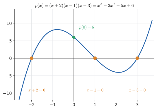
Two important consequences:

A polynomial of degree $n$ has at most $n$ roots. Each root $r$ peels off a factor $(x - r)$ and drops the degree by one; after $n$ peels you are left with a non-zero constant, which has no roots.
Multiplicity. A factor can repeat. In $(x - 1)^2(x + 2)$ the root $1$ has multiplicity 2. Graphically, at a root of even multiplicity the curve touches the axis and turns back; at odd multiplicity it crosses.

Every polynomial has all its roots, somewhere

$x^2 + 1$ has no real roots. But if you allow complex numbers (Chapter 15), the fundamental theorem of algebra (Gauss, 1799) guarantees that every polynomial of degree $n \ge 1$ has exactly $n$ roots counted with multiplicity, so it factors completely into $n$ linear factors. Over the reals, every polynomial factors into linear and irreducible quadratic pieces. And a theorem of Abel and Galois (1820s) shows that, unlike degrees 2, 3 and 4, there is no general formula in radicals for the roots of a degree-5 polynomial. Beyond degree 4, numerical methods are not a convenience but a necessity.

7.6.4. Worked example: using the factor theorem

Show that $(x + 3)$ is a factor of $p(x) = x^3 + 4x^2 + x - 6$, then factor completely.

$(x + 3) = (x - (-3))$, so test $r = -3$:

\[p(-3) = (-27) + 4(9) + (-3) - 6 = -27 + 36 - 3 - 6 = 0 . \checkmark\]

Synthetic division by $r = -3$: bring down $1$; $1(-3) + 4 = 1$; $1(-3) + 1 = -2$; $-2(-3) - 6 = 0$. Quotient $x^2 + x - 2 = (x + 2)(x - 1)$. Therefore $p(x) = (x + 3)(x + 2)(x - 1)$.

7.6.5. Building a polynomial from its roots

The factor theorem also runs forwards. "Find a cubic with roots $1$, $2$, $-4$ and $p(0) = 16$" means $p(x) = k(x - 1)(x - 2)(x + 4)$ for some constant $k$. At $x = 0$: $k(-1)(-2)(4) = 8k = 16$, so $k = 2$. This idea, choosing a polynomial to pass through prescribed points, grows into polynomial interpolation (Lagrange interpolation), the basis of Shamir’s secret-sharing scheme and Reed–Solomon error-correcting codes (Chapter 32).

7.6.6. Where you’d use this

Engineering: is the system stable? The behaviour of a feedback system (a cruise control, a drone’s attitude controller, an amplifier) is governed by the roots of its characteristic polynomial. The system settles down when every root is negative (more precisely, has negative real part). Suppose testing reveals that $s = -1$ is a root of $s^3 + 6s^2 + 11s + 6$. Synthetic division by $(s + 1)$ leaves $s^2 + 5s + 6 = (s + 2)(s + 3)$, so the roots are $-1, -2, -3$: all negative, so the system is stable. Dividing out a known root to shrink the problem is called deflation, and numerical root-finders do it routinely.
Signal processing: designing from the roots. Building a polynomial from chosen roots is how simple digital filters are designed. To block a particular frequency (for example, 50 Hz or 60 Hz mains hum in an audio recording), the designer places a pair of (complex) roots of the filter’s polynomial at the point corresponding to that frequency and multiplies out the factors to get the coefficients the code actually uses.
Checking data. The remainder theorem says the remainder on division by $x - r$ is just $p(r)$. Checksums such as CRCs use the remainder on division by a fixed polynomial as a fingerprint of a message (Section 7.10).

7.7. The rational root theorem

7.7.1. The problem

The factor theorem is only useful if you can find a root. Trying random numbers is hopeless. For polynomials with integer coefficients, the rational root theorem gives a finite list of candidates.

7.7.2. Why it works

Suppose the fraction $p/q$, in lowest terms, is a root of

\[a_n x^n + a_{n-1}x^{n-1} + \cdots + a_1 x + a_0 = 0\]

with integer coefficients. Substitute and multiply through by $q^n$:

\[a_n p^n + a_{n-1} p^{n-1} q + \cdots + a_1 p q^{n-1} + a_0 q^n = 0 .\]

Move the last term across: $a_0 q^n = -p\,(a_n p^{n-1} + \cdots + a_1 q^{n-1})$. The right side is a multiple of $p$, so $p$ divides $a_0 q^n$. But $p$ shares no factor with $q$ (lowest terms), so $p$ must divide $a_0$. The same argument with the first term moved across shows $q$ divides $a_n$.

Rational root theorem

If a polynomial with integer coefficients has a rational root $p/q$ in lowest terms, then $p$ divides the constant term $a_0$ and $q$ divides the leading coefficient $a_n$. For a monic polynomial ($a_n = 1$), every rational root is an integer dividing $a_0$.

Example 44. Procedure — Finding rational roots

Input: a polynomial with integer coefficients and non-zero constant term. (If $a_0 = 0$, factor out $x$ first.)

Steps:

List the divisors $p$ of $a_0$ and the divisors $q$ of $a_n$.
Form all candidates $\pm p/q$ and remove duplicates.
Test candidates (easiest first) by evaluating $p(x)$, ideally by synthetic division, which gives the quotient for free when the remainder is zero.
When a root is found, continue with the quotient (lower degree). Once the quotient is quadratic, factor it or use the quadratic formula.

Output: all rational roots, and a factorisation.

7.7.3. Worked example

Solve $2x^3 - 3x^2 - 11x + 6 = 0$.

Divisors of $a_0 = 6$: $1, 2, 3, 6$. Divisors of $a_n = 2$: $1, 2$. Candidates:

\[\pm 1,\ \pm 2,\ \pm 3,\ \pm 6,\ \pm \tfrac12,\ \pm \tfrac32 .\]

Test $x = 1$: $2 - 3 - 11 + 6 = -6$ ✗. $x = -1$: $-2 - 3 + 11 + 6 = 12$ ✗. $x = 2$: $16 - 12 - 22 + 6 = -12$ ✗. $x = 3$: $54 - 27 - 33 + 6 = 0$ ✓.

Synthetic division by $3$: bring down $2$; $2 \cdot 3 - 3 = 3$; $3 \cdot 3 - 11 = -2$; $-2 \cdot 3 + 6 = 0$. Quotient $2x^2 + 3x - 2$. Factor with $ac = -4$: $4 \cdot (-1) = -4$, $4 + (-1) = 3$:

\[2x^2 + 3x - 2 = 2x^2 + 4x - x - 2 = 2x(x + 2) - (x + 2) = (2x - 1)(x + 2).\]

So $2x^3 - 3x^2 - 11x + 6 = (x - 3)(2x - 1)(x + 2)$, and the roots are $x = 3, \tfrac12, -2$.

from fractions import Fraction

def divisors(n):
    n = abs(n)
    return [d for d in range(1, n + 1) if n % d == 0]

def rational_roots(coeffs):
    """All rational roots of a polynomial with integer coefficients.

    coeffs: highest power first; assumes the constant term is non-zero.
    """
    lead, const = coeffs[0], coeffs[-1]
    candidates = {Fraction(sign * p, q)
                  for p in divisors(const)
                  for q in divisors(lead)
                  for sign in (1, -1)}
    def value(x):
        result = 0
        for c in coeffs:
            result = result * x + c
        return result
    return sorted(r for r in candidates if value(r) == 0)

print(rational_roots([2, -3, -11, 6]))

[Fraction(-2, 1), Fraction(1, 2), Fraction(3, 1)]

Fraction does exact rational arithmetic, so "equals zero" is a reliable test here. With floating point it would not be (Chapter 32).

Limits of the rational root theorem

The theorem gives candidates, not roots; most fail. And it says nothing about irrational roots: $x^3 - 2 = 0$ has candidates $\pm 1, \pm 2$, none of which work, because its only real root is $\sqrt[3]{2}$. When every candidate fails, the polynomial has no rational roots, and you move on to the quadratic formula (degree 2) or numerical methods.

US curriculum

The remainder and factor theorems, the rational root theorem, and the link between zeros and factors are standard Algebra II content (the Common Core standard "A-APR.B: understand the relationship between zeros and factors of polynomials"). Multiplicity and end behaviour return in Precalculus.

7.8. Evaluating polynomials fast: Horner’s method

7.8.1. The problem

Every time a computer evaluates $\sin x$, $e^x$ or $\ln x$ in a math library, it is (after some range reduction) evaluating a carefully chosen polynomial. Graphics shaders evaluate polynomials for every pixel. So: what is the cheapest way to compute $p(x) = a_n x^n + \cdots + a_1 x + a_0$?

7.8.2. Intuition

The obvious way computes each power separately: $x^n$ takes $n - 1$ multiplications, then one more for the coefficient. Summing over all terms, that is about $n(n+1)/2$ multiplications. Reusing powers (compute $x^2$ from $x$, $x^3$ from $x^2$) brings it down to about $2n$. But you can do better by factoring out $x$ repeatedly:

\[\begin{aligned} 2x^3 - 6x^2 + 2x - 1 &= \big(2x^2 - 6x + 2\big)x - 1\\ &= \big((2x - 6)x + 2\big)x - 1 \\ &= \Big(\big((2)x - 6\big)x + 2\Big)x - 1 . \end{aligned}\]

Reading from the inside out: start with the leading coefficient; repeatedly multiply by $x$ and add the next coefficient. That is exactly the synthetic-division row from Section 7.5, and its final value is the remainder on dividing by $x - r$, which by the remainder theorem is $p(r)$. Horner’s method and synthetic division are the same algorithm.

Example 45. Procedure — Horner’s method

Input: coefficients $a_n, \ldots, a_0$ (highest first) and a value $x$.

Steps:

Set $\text{result} \leftarrow a_n$.
For $k = n-1$ down to $0$: $\text{result} \leftarrow \text{result}\times x + a_k$.

Output: $\text{result} = p(x)$. Cost: exactly $n$ multiplications and $n$ additions.

7.8.3. Worked example

Evaluate $p(x) = 2x^3 - 6x^2 + 2x - 1$ at $x = 3$.

Step	Computation	Result
start	\(a_3\)	\(2\)
1	\(2 \times 3 + (-6)\)	\(0\)
2	\(0 \times 3 + 2\)	\(2\)
3	\(2 \times 3 + (-1)\)	\(5\)

Step

Computation

Result

start

$a_3$

$2$

$2 \times 3 + (-6)$

$0$

$0 \times 3 + 2$

$2$

$2 \times 3 + (-1)$

$5$

So $p(3) = 5$. Direct check: $2(27) - 6(9) + 2(3) - 1 = 54 - 54 + 6 - 1 = 5$ ✓. Three multiplications instead of the six needed naively.

def horner(coeffs, x):
    """Evaluate a polynomial at x.

    coeffs lists coefficients from the highest power down:
    [2, -6, 2, -1] means 2x^3 - 6x^2 + 2x - 1.
    """
    result = 0
    for c in coeffs:
        result = result * x + c
    return result

print(horner([2, -6, 2, -1], 3))

(Starting from result = 0 makes the first pass give $0 \cdot x + a_n = a_n$, which keeps the loop uniform.)

7.8.4. Operation counts and why they matter

Method (degree \(n\))	Multiplications	Additions
Each power from scratch	\(n(n+1)/2\)	\(n\)
Running power \(x^k = x^{k-1}\cdot x\)	\(2n - 1\)	\(n\)
Horner	\(n\)	\(n\)

Method (degree $n$)

Multiplications

Additions

Each power from scratch

$n(n+1)/2$

$n$

Running power $x^k = x^{k-1}\cdot x$

$2n - 1$

$n$

Horner

$n$

For degree 10 that is 55 versus 19 versus 10 multiplications. Horner is provably optimal for general polynomials (Ostrowski 1954, Pan 1966): no algorithm can evaluate an arbitrary degree-$n$ polynomial with fewer than $n$ multiplications. Modern CPUs have a fused multiply–add (FMA) instruction computing $ax + b$ in one step with one rounding, and Horner’s loop is nothing but a chain of FMAs. Horner is also usually more accurate in floating point, because it avoids computing huge powers that are then partially cancelled.

Computer-science connection: Horner is everywhere

Parsing numbers. Converting the string "4721" to an integer is n = n*10 + digit in a loop: Horner’s method evaluating the polynomial $4x^3 + 7x^2 + 2x + 1$ at $x = 10$. A number written in base $b$ is a polynomial evaluated at $b$.
Hashing strings. Java’s String.hashCode() is $s_0 \cdot 31^{n-1} + s_1 \cdot 31^{n-2} + \cdots + s_{n-1}$ (mod $2^{32}$), computed by Horner with $x = 31$. See Section 7.10.
Math libraries. exp, sin and friends end in a Horner evaluation of a minimax polynomial (Chapter 32).

Horner versus the naive loop

Pick a degree $n$ and a value of $x$. The lab evaluates the polynomial three ways, counts multiplications, and (in floating point, for polynomials like $(x - 1)^{10}$ expanded out) plots the error of each method near $x = 1$, where cancellation makes the expanded form noisy whichever way you evaluate it: the naive method is worst and Horner is somewhat better, while evaluating the factored form $(x - 1)^{10}$ directly stays accurate.

Try it: Horner versus the naive loop

Horner, and the people before him

William George Horner published the method in 1819, but it was known to Paolo Ruffini a few years earlier, to Isaac Newton in the 1660s, and to Chinese mathematicians (Qin Jiushao, 1247) centuries before that, who used it as part of a method for extracting roots numerically. It is a good example of an algorithm being named after someone who popularised it in the West.

7.9. Rational expressions

7.9.1. The problem

A cyclist rides 30 km to a town at speed $v$ km/h and returns at $v + 5$ km/h. Total time:

\[T(v) = \frac{30}{v} + \frac{30}{v + 5}.\]

To work with this (solve $T = 5$, say) you need to combine fractions whose numerators and denominators are polynomials. These are rational expressions, and they behave exactly like the numerical fractions of Chapter 2, with one extra hazard: the denominator can be zero for some values of the variable.

Rational expression

A rational expression is a quotient of two polynomials, $\dfrac{P(x)}{Q(x)}$ with $Q$ not the zero polynomial. "Rational" here means "ratio", as in rational numbers $p/q$.

Domain

The domain of an expression is the set of values of the variable for which it is defined. For a rational expression, that is every real number except the roots of the denominator. The domain of $\dfrac{x + 1}{x^2 - 4}$ is all real $x$ except $x = \pm 2$, written $x \neq \pm 2$.

7.9.2. Simplifying: cancel factors, never terms

Just as $\frac{6}{8} = \frac{2 \cdot 3}{2 \cdot 4} = \frac34$, you simplify a rational expression by factoring numerator and denominator and cancelling common factors:

\[\begin{aligned} \frac{x^2 - 4}{x^2 - x - 2} &= \frac{(x - 2)(x + 2)}{(x - 2)(x + 1)} &&\text{(factor both)}\\ &= \frac{x + 2}{x + 1}, \qquad x \neq 2,\ x \neq -1. &&\text{(cancel } (x - 2)\text{)} \end{aligned}\]

The restriction $x \neq 2$ must be carried along: the original expression is undefined at $x = 2$ (it is $0/0$), even though the simplified one is not. The two expressions are equal on the original domain, and only there.

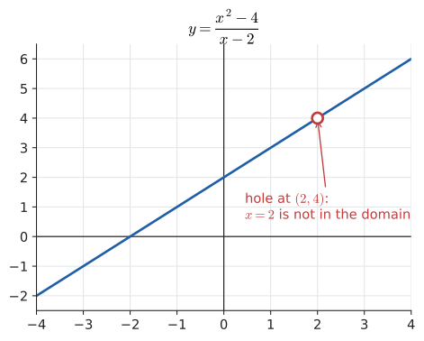
Graph of the line y equals x plus 2 with an open circle at the point 2, 4 indicating a hole where the original expression is undefined

Figure 52. Cancelling a factor leaves a hole

The simplest case shows the picture. Graphically, $\frac{x^2 - 4}{x - 2}$ is the line $y = x + 2$ with a single point punched out at $(2, 4)$: a removable discontinuity, or hole. The example above behaves the same way: $\frac{x + 2}{x + 1}$ with a hole at $(2, \tfrac43)$. A factor that does not cancel from the denominator produces a vertical asymptote instead; that story is told in Chapter 11 and Chapter 16.

Example 46. Procedure — Simplifying a rational expression

Input: $P(x)/Q(x)$.

Steps:

Factor $P$ and $Q$ completely.
Record the domain restriction: every root of $Q$ (from the factored form, before cancelling).
Cancel factors common to numerator and denominator.
State the simplified expression together with the restrictions.

Output: an equivalent expression in lowest terms, valid on the stated domain.

7.9.3. Arithmetic with rational expressions

All four operations follow the fraction rules from Chapter 2:

Multiply: numerators times numerators, denominators times denominators, then cancel.
Divide: multiply by the reciprocal (and add a restriction: the divisor cannot be zero either).
Add/subtract: rewrite over a least common denominator (LCD): the product of every distinct factor of the denominators, each to the highest power it appears.

Worked example (addition).

\[\begin{aligned} \frac{1}{x - 1} + \frac{2}{x + 1} &= \frac{1\cdot(x + 1)}{(x - 1)(x + 1)} + \frac{2\cdot(x - 1)}{(x + 1)(x - 1)} &&\text{(LCD } (x-1)(x+1)\text{)}\\ &= \frac{x + 1 + 2x - 2}{(x - 1)(x + 1)} &&\text{(add numerators)}\\ &= \frac{3x - 1}{x^2 - 1}, \qquad x \neq \pm 1. \end{aligned}\]

Worked example (multiplication and division).

\[\begin{aligned} \frac{x^2 - 9}{x^2 + x} \div \frac{x - 3}{x} &= \frac{x^2 - 9}{x^2 + x} \cdot \frac{x}{x - 3} &&\text{(multiply by reciprocal)}\\ &= \frac{(x - 3)(x + 3)}{x(x + 1)} \cdot \frac{x}{x - 3} &&\text{(factor)}\\ &= \frac{x + 3}{x + 1}, \qquad x \neq 0,\ -1,\ 3. &&\text{(cancel } x \text{ and } (x - 3)\text{)} \end{aligned}\]

The restrictions come from every denominator that ever appeared, including the divisor’s numerator $x - 3$ (dividing by zero is not allowed).

Back to the cyclist. Setting $T(v) = 5$ and multiplying both sides by the LCD $v(v + 5)$:

\[\begin{aligned} 30(v + 5) + 30v &= 5v(v + 5)\\ 60v + 150 &= 5v^2 + 25v\\ 0 &= 5v^2 - 35v - 150 = 5(v^2 - 7v - 30) = 5(v - 10)(v + 3). \end{aligned}\]

So $v = 10$ km/h (the root $v = -3$ is mathematically valid but physically meaningless). Check: $30/10 + 30/15 = 3 + 2 = 5$ ✓. Notice that the rational equation became a quadratic: the subject of the next chapter.

Cancelling terms instead of factors

$\dfrac{x + 6}{x + 3} \neq \dfrac{6}{3} = 2$ and $\dfrac{x^2 + 9}{x + 3} \neq x + 3$. You may only cancel things that multiply the whole numerator and the whole denominator. Test with $x = 1$: $\frac{7}{4} \neq 2$. A second trap: multiplying an equation by an expression containing the variable can introduce extraneous solutions that make an original denominator zero. Always check solutions against the domain.

7.9.4. Where you’d use this

Rational expressions appear whenever rates, shares or reciprocals are combined.

Average speed. Drive to a town at 60 km/h and back at 40 km/h. The average speed is not 50. For a one-way distance $d$, the total time is $\frac{d}{60} + \frac{d}{40}$, so the average is $\dfrac{2d}{d/60 + d/40} = \dfrac{2}{1/60 + 1/40} = \dfrac{2 \cdot 60 \cdot 40}{60 + 40} = 48$ km/h. The $d$ cancels, and simplifying the general version gives the harmonic mean $\frac{2ab}{a + b}$.
Physics. Resistors in parallel combine as $\frac{1}{R} = \frac{1}{R_1} + \frac{1}{R_2}$, i.e. $R = \frac{R_1 R_2}{R_1 + R_2}$: 6 Ω and 3 Ω in parallel give $\frac{18}{9} = 2$ Ω. The thin-lens equation $\frac{1}{f} = \frac{1}{u} + \frac{1}{v}$ has the same shape.
Computing. Amdahl’s law says that if a fraction $p$ of a program’s work can be parallelised over $n$ processors, the speed-up is $S(n) = \dfrac{1}{(1 - p) + p/n}$. With $p = 0.9$ and 8 cores, $S = 1/(0.1 + 0.1125) \approx 4.7$, not 8, and however many cores you add, $S$ stays below $1/(1 - p) = 10$. In machine learning, the F1 score that balances precision $P$ and recall $R$ is their harmonic mean $\frac{2PR}{P + R}$: a classifier with $P = 0.8$ and $R = 0.5$ scores $0.8/1.3 \approx 0.62$.

US curriculum

Simplifying and combining rational expressions, and solving rational equations with extraneous-solution checks, are core Algebra II topics. Holes and asymptotes of rational functions are developed in Precalculus.

7.10. Computer-science connections: hashing and checksums

7.10.1. Polynomial rolling hashes

A hash table needs to turn a string into a number. A natural recipe: treat the characters $s_0, s_1, \ldots, s_{m-1}$ (as character codes) as the coefficients of a polynomial and evaluate it at some base $B$, modulo a large prime $M$ to keep the numbers bounded:

\[h(s) = \left(s_0 B^{m-1} + s_1 B^{m-2} + \cdots + s_{m-1}\right) \bmod M .\]

(The notation $a \bmod M$ means the remainder when $a$ is divided by $M$, Python’s a % M; see Chapter 23.) Horner’s method computes this in $m$ steps.

The magic is in sliding the window. To find a pattern of length $m$ inside a long text, you want the hash of every length-$m$ window. Moving the window one place right removes the leading character and appends a new one:

\[h_{\text{new}} = \big( (h_{\text{old}} - s_{\text{out}}\, B^{m-1}) \cdot B + s_{\text{in}} \big) \bmod M .\]

Subtracting the leading term and multiplying by $B$ is exactly the "drop the top coefficient and shift" step of polynomial arithmetic. Each slide costs $O(1)$, so hashing all windows costs $O(n)$ rather than $O(nm)$. This is the Rabin–Karp string-search algorithm:

def find_all(text, pattern, base=256, mod=1_000_000_007):
    """Rabin-Karp substring search using a polynomial rolling hash."""
    m = len(pattern)
    if m > len(text):
        return []
    high = pow(base, m - 1, mod)          # weight of the outgoing character

    def h(s):                              # Horner's method, mod `mod`
        v = 0
        for ch in s:
            v = (v * base + ord(ch)) % mod
        return v

    target, window = h(pattern), h(text[:m])
    hits = []
    for i in range(len(text) - m + 1):
        if window == target and text[i:i + m] == pattern:
            hits.append(i)
        if i + m < len(text):              # slide: drop text[i], add text[i+m]
            window = (window - ord(text[i]) * high) % mod
            window = (window * base + ord(text[i + m])) % mod
    return hits

print(find_all("abracadabra", "abra"))

[0, 7]

Why does a polynomial hash work well? Two different strings collide only if the difference of their polynomials has $B$ as a root modulo $M$. A non-zero polynomial of degree less than $m$ has at most $m - 1$ roots (the counting argument from Section 7.6 works modulo a prime too), so if $B$ is chosen at random, the collision probability is at most $(m - 1)/M$: tiny. Backup and deduplication systems use the same idea (Rabin fingerprints) to find chunk boundaries in huge files.

7.10.2. CRCs: polynomial division with XOR

A cyclic redundancy check (CRC) protects Ethernet frames, ZIP files and PNG images against corruption. It treats the message bits as the coefficients of a polynomial whose coefficients are just $0$ and $1$, with arithmetic done modulo 2: $1 + 1 = 0$. In that world addition and subtraction are both XOR, and there are no carries.

The sender and receiver agree on a generator polynomial $g(x)$ of degree $n$, for instance $x^3 + x + 1$ (bits 1011). To send message $m(x)$:

Multiply by $x^n$ (append $n$ zero bits).
Divide by $g(x)$ using long division, with XOR for subtraction; keep the remainder $r(x)$ ($n$ bits).
Send $m(x)\,x^n + r(x)$ (the message with the remainder appended). Since subtraction is addition mod 2, this is exactly divisible by $g(x)$.

The receiver divides what arrives by $g(x)$: a non-zero remainder means corruption.

def gf2_remainder(bits, gen):
    """Remainder of polynomial division mod 2 (bits highest power first)."""
    bits = list(bits)
    for i in range(len(bits) - len(gen) + 1):
        if bits[i]:                        # leading term present: subtract gen
            for j, g in enumerate(gen):
                bits[i + j] ^= g           # subtraction mod 2 is XOR
    return bits[-(len(gen) - 1):]

msg = [1, 1, 0, 1, 0, 1]
gen = [1, 0, 1, 1]                         # x^3 + x + 1
crc = gf2_remainder(msg + [0, 0, 0], gen)  # multiply by x^3, then divide
sent = msg + crc
print("crc:", crc)
print("check intact:", gf2_remainder(sent, gen))
corrupt = sent.copy()
corrupt[2] ^= 1                            # flip one bit in transit
print("check corrupt:", gf2_remainder(corrupt, gen))

crc: [1, 1, 1]
check intact: [0, 0, 0]
check corrupt: [1, 0, 1]

This is the long-division procedure from Section 7.5 with every subtraction replaced by XOR, which hardware implements with a shift register and a few XOR gates. A flipped bit adds a term $x^k$ to the message polynomial, and the generator is chosen so that no such single term (and no short burst of terms) is divisible by it, so every such error leaves a non-zero remainder.

Polynomials over finite fields

Polynomials with coefficients taken modulo a prime are the backbone of modern coding theory. The QR code on a parcel and the data on a Blu-ray disc use Reed–Solomon codes: the data are coefficients of a polynomial, the transmitted symbols are its values at many points, and because a degree-$k$ polynomial is determined by any $k + 1$ of its values, the receiver can reconstruct the data even if a large fraction of the symbols are scratched or smudged.

Hash collisions by design

Choose a small modulus $M$ (say 101) and a base $B$. Type strings and watch their polynomial hashes; the lab searches for two strings with the same hash and shows the difference polynomial having $B$ as a root mod $M$. Then increase $M$ and watch collisions become rare.

7.11. Interactive tools

Browser tools on the companion website that go with this chapter. Each example link in the chapter opens one of them with that example already set up.

Where floating point bites

7.12. Exercises

(Recognition) For $p(x) = 5 - 3x^4 + x^2 - 7x$, write it in standard form and state the degree, leading coefficient, constant term, and the coefficient of $x^3$.
(Recognition) Which of these are polynomials? (a) $3x^2 - \tfrac{1}{2}x$ (b) $x^{-2} + 1$ (c) $\sqrt{2}\,x^3$ (d) $\sqrt{x} + 1$ (e) $\dfrac{x^2 + 1}{4}$.
(Application) Expand and simplify: (a) $(3x + 2)(2x^2 - x + 4)$ (b) $(2x - 5)^2$ (c) $(x^2 + 3)(x^2 - 3)$.
(Application) Compute $103 \times 97$ and $51^2$ mentally using special products. Show the identity you used.
(Application) Factor completely: (a) $5x^3 - 20x$ (b) $x^2 - 11x + 28$ (c) $3x^2 + 10x - 8$ (d) $x^3 - 3x^2 - 4x + 12$ (e) $8x^3 + 27$.
(Application) Divide $x^4 - 3x^3 + 2x - 5$ by $x - 2$ using synthetic division. State the quotient and remainder and confirm the remainder using the remainder theorem.
(Application) Divide $3x^3 + x^2 - 4$ by $x^2 + 1$ using long division.
(Problem solving) Find all roots of $x^3 - 7x - 6 = 0$, explaining how you found the first one.
(Problem solving) Find $k$ so that $x - 2$ is a factor of $x^3 + kx^2 - 4x + 8$.
(Problem solving) Simplify $\dfrac{x^2 - 5x + 6}{x^2 - 9} \cdot \dfrac{x + 3}{x - 2}$, stating all domain restrictions.
(Problem solving) Solve $\dfrac{x}{x - 2} - \dfrac{4}{x^2 - 4} = 1$. Watch for extraneous solutions.
(Computing) Modify horner to also return the quotient coefficients, turning it into synthetic division. Test it on $2x^3 - 3x^2 + 5$ at $x = 2$.

Answers

$p(x) = -3x^4 + x^2 - 7x + 5$. Degree 4, leading coefficient $-3$, constant term $5$, coefficient of $x^3$ is $0$.
(a) yes (fractional coefficients are fine). (b) no, negative exponent. (c) yes, $\sqrt2$ is just a constant coefficient. (d) no, $\sqrt x = x^{1/2}$. (e) yes, it is $\tfrac14 x^2 + \tfrac14$.
(a) $6x^3 - 3x^2 + 12x + 4x^2 - 2x + 8 = 6x^3 + x^2 + 10x + 8$. (b) $4x^2 - 20x + 25$. (c) difference of squares: $x^4 - 9$.
$103 \times 97 = (100 + 3)(100 - 3) = 10000 - 9 = 9991$. $51^2 = (50 + 1)^2 = 2500 + 100 + 1 = 2601$.
(a) $5x(x^2 - 4) = 5x(x - 2)(x + 2)$. (b) need $mn = 28$, $m + n = -11$: $-4, -7$, so $(x - 4)(x - 7)$. (c) $ac = -24$; $12 \cdot (-2) = -24$, $12 - 2 = 10$: $3x^2 + 12x - 2x - 8 = 3x(x + 4) - 2(x + 4) = (3x - 2)(x + 4)$. (d) grouping: $x^2(x - 3) - 4(x - 3) = (x - 3)(x^2 - 4) = (x - 3)(x - 2)(x + 2)$. (e) sum of cubes with $a = 2x$, $b = 3$: $(2x + 3)(4x^2 - 6x + 9)$.
Coefficients $1, -3, 0, 2, -5$, $r = 2$: $1$;\ $1\cdot2 - 3 = -1$;\ $-1\cdot2 + 0 = -2$;\ $-2\cdot 2 + 2 = -2$;\ $-2\cdot2 - 5 = -9$. Quotient $x^3 - x^2 - 2x - 2$, remainder $-9$. Check: $p(2) = 16 - 24 + 0 + 4 - 5 = -9$ ✓.
$3x^3 \div x^2 = 3x$; $3x(x^2 + 1) = 3x^3 + 3x$; subtract: $x^2 - 3x - 4$. $x^2 \div x^2 = 1$; subtract $x^2 + 1$: $-3x - 5$. Quotient $3x + 1$, remainder $-3x - 5$. Check: $(x^2 + 1)(3x + 1) - 3x - 5 = 3x^3 + x^2 + 3x + 1 - 3x - 5 = 3x^3 + x^2 - 4$ ✓.
Monic, so rational roots divide $6$: try $\pm1, \pm2, \pm3, \pm6$. $p(-1) = -1 + 7 - 6 = 0$ ✓. Synthetic division of $1, 0, -7, -6$ by $-1$: $1, -1, -6 \mid 0$, quotient $x^2 - x - 6 = (x - 3)(x + 2)$. Roots $-1, 3, -2$.
Factor theorem: $p(2) = 0$: $8 + 4k - 8 + 8 = 0$, so $4k = -8$, $k = -2$.
$\dfrac{(x - 2)(x - 3)}{(x - 3)(x + 3)} \cdot \dfrac{x + 3}{x - 2} = 1$, with $x \neq 3, -3, 2$. The whole expression is the constant 1 with three holes.
LCD $(x - 2)(x + 2)$, restrictions $x \neq \pm 2$. Multiply through: $x(x + 2) - 4 = (x - 2)(x + 2)$, so $x^2 + 2x - 4 = x^2 - 4$, giving $2x = 0$, $x = 0$. Allowed, and check: $0 - 4/(-4) = 1$ ✓. (No extraneous root here, but you had to check.)
Collect the intermediate values: out = []; r = 0; for c in coeffs: r = r*x + c; out.append(r); return out[:-1], out[-1]. On [2, -3, 0, 5] at 2 the intermediate values are 2, 1, 2, 9: quotient $2x^2 + x + 2$, remainder $9$, matching the synthetic division example.

7.13. Mastery check

State the degree and leading coefficient of $(2x^2 - 1)^3$ without expanding it.
Expand $(x - 4)(x^2 + 4x + 16)$ and name the pattern.
Factor completely: $2x^4 - 32$.
Factor $10x^2 - 11x - 6$.
Use the rational root theorem and synthetic division to factor $x^3 + 2x^2 - 5x - 6$.
Without dividing, find the remainder when $x^{50} - 3x + 1$ is divided by $x + 1$.
Simplify $\dfrac{x^3 - x}{x^2 + 2x + 1}$ and state its domain.
Evaluate $3x^4 - 2x^3 + x - 7$ at $x = 2$ with Horner’s method, showing each step. How many multiplications did you use?

Decision rule: All eight correct without hesitation → move on to Chapter 8. Missed items 3–5 → rework Section 7.4 and its exercises; factoring fluency is essential for the next chapter. Missed 6 or 8 → reread Section 7.6 and Section 7.8. Missed 7 → reread Section 7.9. Stuck on more than three → work the section exercises first.

Mastery check answers

Leading term of $(2x^2)^3 = 8x^6$: degree 6, leading coefficient 8.
$x^3 + 4x^2 + 16x - 4x^2 - 16x - 64 = x^3 - 64$: difference of cubes $a^3 - b^3 = (a - b)(a^2 + ab + b^2)$ with $a = x$, $b = 4$.
$2(x^4 - 16) = 2(x^2 - 4)(x^2 + 4) = 2(x - 2)(x + 2)(x^2 + 4)$.
$ac = -60$; need sum $-11$: $-15 \cdot 4 = -60$, $-15 + 4 = -11$. $10x^2 - 15x + 4x - 6 = 5x(2x - 3) + 2(2x - 3) = (2x - 3)(5x + 2)$.
Candidates $\pm1, \pm2, \pm3, \pm6$. $p(-1) = -1 + 2 + 5 - 6 = 0$ ✓. Synthetic division of $1, 2, -5, -6$ by $-1$: $1, 1, -6 \mid 0$. $x^2 + x - 6 = (x + 3)(x - 2)$. So $(x + 1)(x - 2)(x + 3)$.
Remainder theorem with $r = -1$: $(-1)^{50} - 3(-1) + 1 = 1 + 3 + 1 = 5$.
$\dfrac{x(x - 1)(x + 1)}{(x + 1)^2} = \dfrac{x(x - 1)}{x + 1}$, domain $x \neq -1$.
Coefficients $3, -2, 0, 1, -7$: $3$;\ $3\cdot2 - 2 = 4$;\ $4 \cdot 2 + 0 = 8$;\ $8\cdot2 + 1 = 17$;\ $17 \cdot 2 - 7 = 27$. Value $27$, using 4 multiplications (one per degree). Check: $48 - 16 + 2 - 7 = 27$ ✓.