Volume 2: Continuous Mathematics · Part V: Calculus
Chapter 18. Using Derivatives: Optimisation, Approximation, and Newton’s Method
In Chapter 17 you built the derivative: the instantaneous rate of change, the slope of the tangent line, and a toolkit of rules for computing it. This chapter puts that machine to work. A single number, \(f'(x)\), turns out to tell you where a function rises and falls, where it peaks, how to build the best box from a sheet of card, how fast a ladder’s top slides down a wall, how to approximate a hard function by an easy one, and — the chapter’s centrepiece — how to solve equations that algebra cannot touch, using Newton’s method. Throughout, the same idea recurs: near any point, a smooth curve looks like its tangent line, and lines are easy.
Why this chapter matters: this is where calculus starts paying rent. Setting a price, sizing a checkpoint interval, dosing a drug, judging how a measurement error spreads through a calculation, computing a square root inside a chip, and training a machine-learning model are all applications of the handful of ideas below.
18.1. What the derivative says about shape
18.1.1. The problem
You are handed a formula — say the profit of a product as a function of its price, or the height of a projectile as a function of time — and asked: where is it largest? Plotting helps, but a plot is only as good as the points you sampled, and it never proves anything. You want a way to read the shape of a graph directly from the formula.
The derivative is exactly that tool. Recall that \(f'(x)\) is the slope of the tangent line at \(x\). Slope has a sign, and the sign is a direction:
-
\(f'(x) > 0\): the tangent tilts upward, so the graph is climbing;
-
\(f'(x) < 0\): the tangent tilts downward, so the graph is falling;
-
\(f'(x) = 0\): the tangent is horizontal — the graph is momentarily level.
18.1.2. Intuition
Walk along a hilly road from left to right. While you climb, your altimeter’s rate of change is positive. At the very top of a hill — for one instant — you are neither climbing nor descending: the rate is zero. Then you start to descend and the rate turns negative. So the summit is betrayed by the rate passing through zero and changing sign from + to −. A valley floor is the reverse: − then 0 then +.
That is the whole idea of this section. Peaks and troughs hide at the places where \(f'\) is zero (or fails to exist), and the sign change of \(f'\) around those places tells you which is which.
18.1.3. Why it works
Why must a smooth function with a positive derivative everywhere on an interval actually be increasing there? Positive slope at every single point feels like it should force the function up, but "slope at a point" is a limit — an instantaneous statement — and "increasing" compares two different points.
The bridge is the Mean Value Theorem: if \(f\) is differentiable on an interval and \(a < b\) are two points in it, then somewhere between them there is a point \(c\) where the tangent slope equals the average slope:
Picture it: draw the chord (secant) from \((a, f(a))\) to \((b, f(b))\); slide a parallel line toward the curve, and it must touch the curve somewhere as a tangent. Now rearrange: \(f(b) - f(a) = f'(c)\,(b-a)\). If \(f'\) is positive everywhere and \(b - a > 0\), the right-hand side is positive, so \(f(b) > f(a)\). The function is increasing. Same argument with signs flipped for decreasing, and with \(f' = 0\) everywhere it says \(f(b) = f(a)\): a function with zero derivative is constant. (That last fact is the reason antiderivatives come with a "+ C" in Chapter 19.)
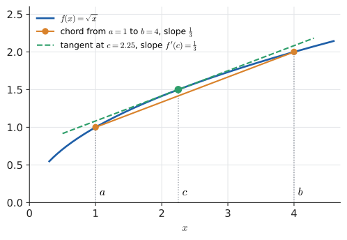
The Mean Value Theorem is also the legal basis of average-speed cameras: if your average speed between two cameras was 62 mph, the theorem guarantees that at some instant your speedometer read exactly 62 mph. Over a 50 mph limit, that is enough for a ticket. Try it: Mean value point for √x.
18.1.4. Vocabulary and notation
|
Increasing and decreasing
A function \(f\) is increasing on an interval if \(a < b\) implies \(f(a) < f(b)\) for any two points in the interval, and decreasing if \(a < b\) implies \(f(a) > f(b)\). Test: \(f' > 0\) on an interval ⇒ increasing there; \(f' < 0\) ⇒ decreasing. |
|
Critical point (stationary point)
A critical point of \(f\) is a point \(c\) in its domain where \(f'(c) = 0\) or \(f'(c)\) does not exist. Where \(f'(c) = 0\) specifically, UK texts say stationary point: the tangent is horizontal. Every local maximum or minimum of a function at an interior point is a critical point — but not every critical point is a maximum or minimum. |
|
Local and global extrema
\(f\) has a local maximum at \(c\) if \(f(c) \ge f(x)\) for all \(x\) near \(c\); a local minimum if \(f(c) \le f(x)\) nearby. A global (or absolute) maximum or minimum compares against every point of the domain. Extremum (plural extrema) means "maximum or minimum". UK texts often say turning point for a local extremum. |
|
Concave up, concave down, inflection point
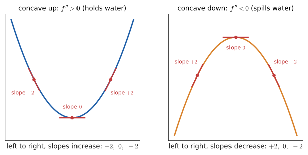
\(f\) is concave up (UK: convex) on an interval where its slope is increasing — the graph bends like a cup, \(\cup\). It is concave down (UK: concave) where its slope is decreasing — a cap, \(\cap\). Test: \(f'' > 0\) ⇒ concave up; \(f'' < 0\) ⇒ concave down. An inflection point is a point on the graph where the concavity changes. |
The UK/US clash in the concavity vocabulary is real and causes confusion: a US textbook’s "concave up" is a British "convex". In optimisation and machine learning the British/European usage wins: a convex function is cup-shaped, and convexity guarantees that any local minimum is a global one.
18.1.5. The method: first and second derivative tests
Input: a differentiable function \(f\) (except possibly at isolated points).
Steps:
-
Compute \(f'(x)\) and factor it as far as possible.
-
Find the critical points: solve \(f'(x) = 0\), and list points where \(f'\) is undefined but \(f\) is defined.
-
Mark the critical points on a number line. They split it into intervals.
-
In each interval pick a test point and find the sign of \(f'\) there (factored form makes this a sign-counting exercise).
-
Classify each critical point \(c\):
-
sign changes \(+ \to -\): local maximum;
-
sign changes \(- \to +\): local minimum;
-
no sign change: neither (a level spot on a rising or falling stretch).
-
Output: the intervals of increase and decrease, and the classification of every critical point.
The second derivative gives a quicker test at a stationary point \(c\) (where \(f'(c) = 0\)):
-
\(f''(c) > 0\): concave up at \(c\) — a cup — so \(c\) is a local minimum;
-
\(f''(c) < 0\): concave down — a cap — so \(c\) is a local maximum;
-
\(f''(c) = 0\): the test says nothing. Fall back on the first derivative test.
18.1.6. Worked example: a cubic
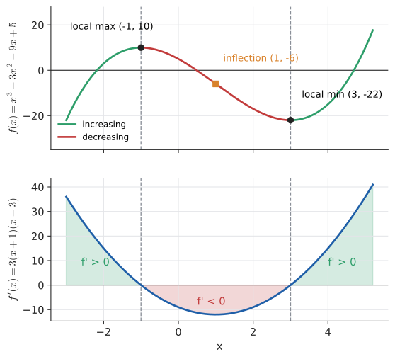
Find and classify the critical points of \(f(x) = x^3 - 3x^2 - 9x + 5\), find where it is concave up and down, and locate its inflection point. Try it: Differentiate the cubic.
Step 1 — differentiate and factor.
Step 2 — critical points. \(f'(x) = 0\) when \(x = -1\) or \(x = 3\). \(f'\) is a polynomial, defined everywhere, so there are no others.
Step 3 — sign chart. The critical points split the line into three intervals. Test one point in each:
| Interval | test \(x\) | \(x+1\) | \(x-3\) | sign of \(f'(x) = 3(x+1)(x-3)\) |
|---|---|---|---|---|
\(x < -1\) |
\(-2\) |
\(-\) |
\(-\) |
\(+\) (increasing) |
\(-1 < x < 3\) |
\(0\) |
\(+\) |
\(-\) |
\(-\) (decreasing) |
\(x > 3\) |
\(4\) |
\(+\) |
\(+\) |
\(+\) (increasing) |
Step 4 — classify and evaluate.
Step 5 — check with the second derivative. \(f''(x) = 6x - 6\).
Step 6 — concavity and inflection. \(f''(x) = 6(x - 1)\) is negative for \(x < 1\) and positive for \(x > 1\). The concavity changes at \(x = 1\), where \(f(1) = 1 - 3 - 9 + 5 = -6\). The inflection point is \((1, -6)\) — exactly halfway between the two turning points, as it always is for a cubic.
18.1.7. Failure modes
|
Three traps with critical points
|
18.1.8. Where you’d use this
-
Medicine: peak drug level. After a tablet, the concentration in the blood is often modelled as \(C(t) = 20t\,e^{-0.5t}\) mg/L (\(t\) in hours). Product rule: \(C'(t) = 20e^{-0.5t}(1 - 0.5t)\), which is zero only at \(t = 2\); the sign goes \(+ \to -\), so the peak is at 2 hours, \(C(2) = 40/e \approx 14.7\) mg/L. Pharmacologists call these \(t_{\max}\) and \(C_{\max}\), and they decide dosing intervals.
-
Everyday: reading an epidemic or sales curve. On a graph of total cases (or total downloads of an app), the inflection point is the moment the daily count peaks: before it the curve is concave up (each day worse than the last), after it concave down (still rising, but more slowly). "We have passed the inflection point" is a claim about the sign of \(f''\).
-
Engineering. A beam’s bending moment is largest where its derivative, the shear force, is zero; structural engineers find the critical section with exactly this first derivative test.
-
Computing. Peak detection in signals (finding heartbeats in an ECG trace, or onsets in audio) looks for sign changes of the discrete slope \(y_{k+1} - y_k\), the first derivative test applied to samples. And optimisers check convexity (\(f'' \ge 0\) everywhere) because a convex loss has no traps: every local minimum is global.
18.2. Curve sketching as a procedure
You have a function and want an honest picture of it — not a plot from a few sampled points that might miss a wiggle, but a sketch whose every feature is justified. As a programmer you will recognise what follows: it is a pipeline that collects facts and then renders them.
Input: a formula for \(f\).
Steps:
-
Domain. Where is \(f\) defined? (Watch for division by zero, even roots of negatives, logarithms of non-positives.)
-
Intercepts. \(y\)-intercept: \(f(0)\). \(x\)-intercepts: solve \(f(x) = 0\) if feasible.
-
Symmetry. Even (\(f(-x) = f(x)\), mirror in the \(y\)-axis) or odd (\(f(-x) = -f(x)\), rotational symmetry about the origin)?
-
Asymptotes and end behaviour. Limits as \(x \to \pm\infty\), and at any excluded points (Chapter 16).
-
First derivative. Critical points; intervals of increase/decrease; classify local extrema.
-
Second derivative. Intervals of concavity; inflection points.
-
Tabulate the key points with their \(y\)-values.
-
Draw: plot the key points and connect them, obeying the rise/fall and bend information on each interval.
Output: a sketch with every max, min, inflection, intercept and asymptote correctly placed.
18.2.1. Worked example
Sketch \(f(x) = x^4 - 4x^3\).
-
Domain: all real \(x\) (a polynomial).
-
Intercepts: \(f(0) = 0\). Solve \(x^4 - 4x^3 = x^3(x - 4) = 0\): \(x = 0\) or \(x = 4\).
-
Symmetry: \(f(-x) = x^4 + 4x^3\), which is neither \(f(x)\) nor \(-f(x)\). No symmetry.
-
End behaviour: the leading term \(x^4\) dominates, so \(f(x) \to +\infty\) as \(x \to \pm\infty\).
-
First derivative:
\[f'(x) = 4x^3 - 12x^2 = 4x^2(x - 3).\]Critical points: \(x = 0\) and \(x = 3\). Signs: \(4x^2 \ge 0\) always, so the sign of \(f'\) is the sign of \(x - 3\) (except at \(x = 0\)): negative for \(x < 3\), positive for \(x > 3\). So \(f\) decreases on \((-\infty, 3)\) and increases on \((3, \infty)\). At \(x = 3\): \(- \to +\), a local (in fact global) minimum, \(f(3) = 81 - 108 = -27\). At \(x = 0\): no sign change — a stationary point that is not an extremum.
-
Second derivative:
\[f''(x) = 12x^2 - 24x = 12x(x - 2).\]Zero at \(x = 0\) and \(x = 2\). Signs: positive for \(x < 0\), negative on \((0, 2)\), positive for \(x > 2\). Concavity changes at both, so both are inflection points: \((0, 0)\) and \((2, 16 - 32) = (2, -16)\).
-
Key points:
\(x\) \(f(x)\) feature \(0\)
\(0\)
intercept; stationary inflection point (flat, bending changes)
\(2\)
\(-16\)
inflection point (falling, cap turns to cup)
\(3\)
\(-27\)
global minimum
\(4\)
\(0\)
intercept
-
Draw: come down from the upper left in a cup shape, flatten to a horizontal tangent at the origin while switching to a cap, keep falling and switch back to a cup at \((2,-16)\), bottom out at \((3,-27)\), rise through \((4, 0)\) and up to the right.
Notice what the procedure caught that random sampling might miss: the origin is flat but not a turning point. Point-sampling plots tend to show it as a slight kink or not at all.
18.3. Optimisation
18.3.1. The problem
"Optimisation" is mathematics for the question every engineer asks: what is the best choice? The cheapest design, the shortest route, the highest throughput, the smallest error. In the single-variable form it reads: find the value of \(x\) in some allowed set that makes a quantity \(f(x)\) as large (or as small) as possible.
18.3.2. Intuition and why it works
A smooth function on a closed interval \(\left[a, b\right]\) has to achieve both a highest and a lowest value somewhere — this is the Extreme Value Theorem. The highest point can only be in one of two kinds of place:
-
at an endpoint \(a\) or \(b\) (the function might just keep rising until it is stopped by the boundary), or
-
at an interior point where the graph turns over — and there, if \(f\) is differentiable, the tangent must be horizontal: \(f'(c) = 0\).
Why horizontal? If \(f'(c) > 0\) at an interior point you could step slightly right and go higher; if \(f'(c) < 0\) you could step slightly left and go higher. Either way \(c\) would not be the top. Only \(f'(c) = 0\) (or a point where \(f'\) fails to exist) survives. This is Fermat’s theorem on stationary points, and it reduces an infinite search over every \(x\) to a short list of candidates.
|
Objective function and constraint
In an optimisation problem, the objective function is the quantity you want to maximise or minimise (volume, area, cost, error). A constraint is a condition the variables must satisfy (fixed fence length, fixed volume). The feasible set or domain is the set of values satisfying all constraints. The best value of the objective is the optimum; the \(x\) achieving it is the optimiser (\(\arg\max\) or \(\arg\min\)). |
18.3.3. The method
Input: a situation described in words.
Steps:
-
Draw a picture and name the quantities with letters, including units.
-
Write the objective — the quantity to optimise — as a formula. It will often involve two or more variables.
-
Use the constraint to eliminate all but one variable, giving the objective as \(f(x)\).
-
State the domain of \(x\) from the physical situation (lengths positive, can’t cut more than the sheet, …).
-
Differentiate, solve \(f'(x) = 0\), and list critical points in the domain.
-
Compare candidates: evaluate \(f\) at each critical point and at the endpoints of the domain (closed-interval method); or, on an open domain, confirm with the first or second derivative test.
-
Answer the question that was asked — in words, with units. (Often it asks for the dimensions, not the optimal value, or both.)
Output: the optimal choice and the optimal value.
18.3.4. Worked example 1: the open box
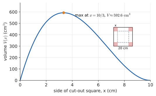
A square sheet of card is 20 cm on each side. You cut an equal square of side \(x\) from each corner and fold up the flaps to make an open-topped box. What \(x\) gives the largest volume? Try it: Design the open box; Graph the box volume.
Picture and names. After cutting, the base is a square of side \(20 - 2x\) (you lose \(x\) at each end), and the height is \(x\).
Objective. Volume = base area × height:
There was only one free variable to begin with, so no constraint is needed to eliminate anything.
Domain. \(x\) must be positive, and \(20 - 2x\) must be positive, so \(0 \le x \le 10\) (allowing the degenerate endpoint boxes, which have zero volume).
Differentiate. Use the product rule with \(u = x\), \(v = (20 - 2x)^2\), so \(u' = 1\) and, by the chain rule, \(v' = 2(20 - 2x)\cdot(-2) = -4(20 - 2x)\):
Critical points. \(V'(x) = 0\) when \(20 - 2x = 0\) (\(x = 10\), an endpoint) or \(20 - 6x = 0\) (\(x = 10/3 \approx 3.333\)).
Compare candidates.
Answer. Cut squares of side \(10/3 \approx 3.33\) cm. The box is \(13.33 \times 13.33 \times 3.33\) cm and holds about \(593\ \text{cm}^3\).
18.3.5. Worked example 2: fencing along a river
A farmer has 200 m of fencing to enclose a rectangular field along a straight river. No fence is needed along the river. What dimensions maximise the area?
Names. Let \(x\) be the length of each of the two sides perpendicular to the river and \(y\) the side parallel to it.
Objective: \(A = xy\). Constraint: fence used \(= 2x + y = 200\).
Eliminate. \(y = 200 - 2x\), so
Differentiate and solve.
Check. \(A''(x) = -4 < 0\), so concave down everywhere: \(x = 50\) is the global maximum. (Endpoints give \(A(0) = A(100) = 0\).)
Answer. \(x = 50\) m, \(y = 200 - 100 = 100\) m, area \(5000\ \text{m}^2\). The side along the river is twice each of the other sides.
Alternative approach. \(A(x) = 200x - 2x^2\) is a downward parabola; completing the square (Chapter 8) gives \(A = -2(x - 50)^2 + 5000\), so the vertex is at \(x = 50\) — no calculus needed. For quadratics, the vertex formula is the quicker method. Calculus earns its keep when the objective is not a quadratic, as in the next example.
18.3.6. Worked example 3: minimal cost of a can
A drinks company wants a closed cylindrical can holding \(500\ \text{cm}^3\). Metal costs the same per square centimetre everywhere, so minimising cost means minimising surface area. What radius and height should they use? Try it: Find the cheapest can.
Names. Radius \(r\), height \(h\), both in cm.
Objective. Surface area = two circular ends + the curved side (which unrolls into a rectangle of width \(2\pi r\), height \(h\)):
Constraint. \(\pi r^2 h = 500\), so \(h = \dfrac{500}{\pi r^2}\).
Eliminate.
Differentiate. Write \(1000/r = 1000 r^{-1}\):
Check. \(S''(r) = 4\pi + 2000/r^3 > 0\) for all \(r > 0\): concave up on the whole domain, so this single critical point is the global minimum. (The domain \(r > 0\) is open — there are no endpoints to check — but as \(r \to 0^+\) or \(r \to \infty\), \(S \to \infty\), confirming a minimum in between.)
Height. Here is the elegant part. From \(r^3 = 250/\pi\) we get \(\pi r^3 = 250\), so
Answer. \(r \approx 4.30\) cm, \(h \approx 8.60\) cm, surface area \(S \approx 348.7\ \text{cm}^2\). The cheapest can is exactly as tall as it is wide. (Real drinks cans are taller and thinner, because thicker metal is used for the ends, the ends are more expensive to form, and a tall can is easier to hold — change the cost per unit area of the ends in exercise 6 and watch the optimum move.)
18.3.7. Alternative approaches and choosing a method
-
Algebra alone: for quadratic objectives, the vertex of a parabola (completing the square) is fastest. For products with a fixed sum, the AM–GM inequality (\(\sqrt{ab} \le \tfrac{a+b}{2}\), equality when \(a = b\)) solves many problems in one line.
-
Calculus: the general tool for any differentiable objective in one variable.
-
Numerical search: when \(f'(x) = 0\) can’t be solved by hand — apply Newton’s method (Section 18.10) to \(f'\), or evaluate \(f\) on a fine grid. For many variables, gradient descent (Section 18.11).
Choose the lightest tool that works. If the objective is a quadratic, don’t differentiate it twice and run the second-derivative test; just find the vertex.
|
Classic optimisation mistakes
|
18.3.8. Where you’d use this
-
Everyday and business: setting a price. A small company sells phone cases that cost £10 each to make. At price \(p\) pounds it sells \(q = 1000 - 20p\) a month. Profit is \(P(p) = (p - 10)(1000 - 20p)\), so \(P'(p) = (1000 - 20p) - 20(p - 10) = 1200 - 40p\), zero at \(p = 30\). At £30 it sells 400 cases for a profit of \(20 \times 400 = 8000\) pounds a month; at £25 or £35 the profit is only £7500. Economists phrase the same calculation as "marginal revenue equals marginal cost".
-
Engineering: minimum material for a given strength (the can and box above are the toy versions); optimal beam cross-sections.
-
Physics: light travels the path of least time (Fermat’s principle); setting the derivative of travel time to zero gives Snell’s law of refraction, the rule behind lenses and fibre optics.
-
Computing: how often to checkpoint. A long computation saves a checkpoint every \(\tau\) seconds; each save costs \(C\) seconds, and on a crash you lose on average half an interval. With failures every \(M\) seconds on average, the time wasted per second is about \(W(\tau) = \frac{C}{\tau} + \frac{\tau}{2M}\). Then \(W'(\tau) = -\frac{C}{\tau^2} + \frac{1}{2M} = 0\) gives \(\tau = \sqrt{2CM}\) (Young’s formula). For a 60-second checkpoint and one failure a day (\(M = 86\,400\) s), \(\tau = \sqrt{2 \cdot 60 \cdot 86\,400} \approx 3220\) s: checkpoint about every 54 minutes. The same "one cost falls, one rises" shape governs cache sizes, batch sizes and retry timeouts.
|
The bees knew first
Pappus of Alexandria (4th century) remarked that bees build hexagonal cells because, among shapes that tile the plane, the hexagon encloses the most honey for the least wax. This "honeycomb conjecture" — that the regular hexagonal tiling has the least total perimeter for cells of a given area — was finally proved by Thomas Hales in 1999. Optimisation questions are easy to state and can be very hard to settle. |
|
Box designer
Drag a slider for the cut size \(x\) on a 20 cm sheet and watch a 3-D box fold up, with its volume plotted live as a point on the \(V(x)\) curve. A second slider changes the sheet to a rectangle (\(a \times b\)); see the optimum move, and compare it with the root of \(V'(x) = 0\) found by the quadratic formula. |
18.4. Exercises: shape and optimisation
-
(Recognition) At a point \(c\), \(f'(c) = 0\) and \(f''(c) = 5\). What can you conclude? What if \(f''(c) = 0\)?
-
(Application) Find and classify the critical points of \(g(x) = x^3 - 12x\). Where is \(g\) concave up?
-
(Application) Find the global maximum and minimum of \(h(x) = x^3 - 3x\) on the interval \(\left[0, 3\right]\).
-
(Application) Two positive numbers add to 20. Which pair has the largest product?
-
(Problem solving) A rectangle has perimeter 400 m (fenced on all four sides). Show that the area is maximised by a square.
-
(Problem solving) Redo the can problem with the ends costing twice as much per \(\text{cm}^2\) as the side. Show that the optimal can now has \(h = 4r\). Try it: Ends cost double: h = 4r.
Answers
-
\(f''(c) > 0\) means concave up at a stationary point: a local minimum. If \(f''(c) = 0\) the second derivative test is inconclusive; use the first derivative test (e.g. \(x^4\), \(-x^4\), \(x^3\) at 0 give min, max, neither).
-
\(g'(x) = 3x^2 - 12 = 3(x - 2)(x + 2)\), so critical points \(x = \pm 2\). \(g''(x) = 6x\): \(g''(-2) = -12 < 0\), so local max \(g(-2) = -8 + 24 = 16\); \(g''(2) = 12 > 0\), so local min \(g(2) = 8 - 24 = -16\). Concave up where \(6x > 0\), i.e. \(x > 0\); inflection at \((0, 0)\).
-
\(h'(x) = 3x^2 - 3 = 3(x-1)(x+1)\); in \(\left[0,3\right]\) the only critical point is \(x = 1\). Candidates: \(h(0) = 0\), \(h(1) = 1 - 3 = -2\), \(h(3) = 27 - 9 = 18\). Global max 18 at \(x = 3\) (an endpoint), global min \(-2\) at \(x = 1\).
-
Numbers \(x\) and \(20 - x\); \(P(x) = 20x - x^2\), \(P'(x) = 20 - 2x = 0\) gives \(x = 10\); \(P'' = -2 < 0\). Both numbers are 10, product 100.
-
Sides \(x\) and \(y\) with \(2x + 2y = 400\), so \(y = 200 - x\) and \(A(x) = x(200 - x) = 200x - x^2\). \(A'(x) = 200 - 2x = 0 \Rightarrow x = 100\), so \(y = 100\): a square, area \(10\,000\ \text{m}^2\). \(A'' = -2 < 0\) confirms a maximum.
-
Cost \(C = 2\cdot(2\pi r^2) + 2\pi r h\) (in units of the side price). With \(h = 500/(\pi r^2)\): \(C(r) = 4\pi r^2 + 1000/r\), \(C'(r) = 8\pi r - 1000/r^2 = 0 \Rightarrow r^3 = 125/\pi\), i.e. \(\pi r^3 = 125\). Then \(h = 500/(\pi r^2) = 4\cdot 125/(\pi r^2) = 4\pi r^3/(\pi r^2) = 4r\). \(r \approx 3.41\) cm, \(h \approx 13.66\) cm — taller and thinner, like a real can.
18.5. Related rates
18.5.1. The problem
Air is pumped into a spherical balloon at a steady \(100\ \text{cm}^3\) per second. How fast is the radius growing when the radius is 10 cm? You know one rate (volume per second) and want another (radius per second). The two quantities are tied together by a formula, \(V = \tfrac{4}{3}\pi r^3\), and that link forces their rates to be tied together too.
18.5.2. Intuition and why it works
When several quantities all change with time, each is a function of \(t\). If an equation relates them at every instant, you can differentiate both sides of the equation with respect to \(t\) — the two sides are equal functions of time, so their rates of change are equal. The chain rule (Chapter 17) does the work: the derivative of \(r^3\) with respect to time is \(3r^2 \cdot \frac{dr}{dt}\), "the rate \(V\) changes per unit of \(r\), times the rate \(r\) changes per unit of time". This is implicit differentiation with time as the hidden variable.
Input: a situation with several changing quantities, one known rate, one wanted rate, and the "snapshot" values at the instant of interest.
Steps:
-
Draw a picture; name every changing quantity as a function of time.
-
Write down the known rate and the wanted rate as derivatives (e.g. \(\frac{dV}{dt} = 100\), want \(\frac{dr}{dt}\)).
-
Find an equation linking the quantities that holds at all times.
-
Differentiate both sides with respect to \(t\) (chain rule on every changing quantity).
-
Only now substitute the snapshot values, and solve for the wanted rate.
-
State the answer with units and sign (negative means decreasing).
Output: the wanted rate at the given instant.
18.5.3. Worked example 1: the balloon
Known: \(\frac{dV}{dt} = 100\ \text{cm}^3/\text{s}\). Wanted: \(\frac{dr}{dt}\) when \(r = 10\) cm. Link: \(V = \tfrac{4}{3}\pi r^3\).
Notice that \(4\pi r^2\) is the balloon’s surface area: the new air is spread as a thin shell over the whole surface, so the bigger the balloon, the slower the radius grows.
18.5.4. Worked example 2: the sliding ladder (a Mechanics classic)
A 5 m ladder leans against a vertical wall. Its foot slides away from the wall at \(0.5\) m/s. How fast is the top sliding down the wall when the foot is 3 m from the wall?
Names. \(x(t)\): distance of the foot from the wall; \(y(t)\): height of the top. Known: \(\frac{dx}{dt} = 0.5\). Wanted: \(\frac{dy}{dt}\) when \(x = 3\). Link (Pythagoras, true at all times): \(x^2 + y^2 = 25\).
Snapshot: when \(x = 3\), \(y = \sqrt{25 - 9} = 4\).
The top slides down (negative sign) at \(0.375\) m/s. As the top approaches the ground (\(y \to 0\)), \(\frac{dy}{dt} = -\frac{x}{y}\frac{dx}{dt}\) grows without bound — the model breaks down because in reality the ladder’s top leaves the wall.
|
Substituting too early
Never plug in the snapshot values before differentiating. If you wrote \(x = 3\) into \(x^2 + y^2 = 25\) first, you would get \(9 + y^2 = 25\), and differentiating that says \(2y\frac{dy}{dt} = 0\) — nonsense, because you have frozen \(x\) at one instant and thrown its rate away. Differentiate the general relationship, then substitute. |
18.5.5. Where you’d use this
-
Navigation and radar. A radar dish measures how fast the distance to an aircraft changes, not the aircraft’s speed. A plane at 10 km altitude flies level at 800 km/h straight towards a point above the radar. With horizontal distance \(x\) and slant distance \(s\), \(s^2 = x^2 + 10^2\), so \(s\frac{ds}{dt} = x\frac{dx}{dt}\). When \(x = 24\) km, \(s = 26\) km, and the radar sees \(\frac{ds}{dt} = \frac{24}{26}\times(-800) \approx -738\) km/h: the closing speed is less than the true speed, and the related-rates equation is how the system corrects for it. Police speed guns aimed from the roadside have the same "cosine error", which always underestimates your speed.
-
Medicine. Doctors track a tumour by its diameter on a scan, but treatment depends on volume. For a sphere of diameter \(D\), \(V = \frac{\pi}{6}D^3\), so \(\frac{dV}{dt} = \frac{\pi}{2}D^2\frac{dD}{dt}\). A 2 cm tumour growing 1 mm a month is adding \(\frac{\pi}{2}(4)(0.1) \approx 0.63\) cm³ a month, and the same diametric growth at 4 cm means four times the volume growth.
-
Computing. In games and animation, a camera tracking a moving target must turn at the rate \(\frac{d\theta}{dt}\) implied by the target’s speed and distance (differentiate \(\tan\theta = y/x\)); a target passing close by makes the required turn rate spike, which is why fast fly-bys look jerky without smoothing.
18.6. Linear approximation and differentials
18.6.1. The problem
Without a calculator, what is \(\sqrt{4.1}\)? You know \(\sqrt{4} = 2\) exactly, and \(4.1\) is very close to 4. Surely \(\sqrt{4.1}\) is just a little more than 2 — but how much more?
18.6.2. Intuition
Zoom in on any smooth curve far enough and it looks straight — it looks like its tangent line. So near a point \(a\) where you know everything, replace the curve by its tangent line and evaluate the line instead. Lines are trivial to evaluate.
18.6.3. Why it works
The tangent line at \(x = a\) passes through \((a, f(a))\) with slope \(f'(a)\). Point-slope form (Chapter 5) gives
This \(L\) is the linearisation of \(f\) at \(a\). Because \(f'(a)\) is the limit of the slopes \(\frac{f(x) - f(a)}{x - a}\), the gap \(f(x) - L(x)\) shrinks faster than \(x - a\) itself as \(x \to a\). For twice-differentiable functions the error is roughly \(\tfrac{1}{2}f''(a)(x-a)^2\): halve the distance, quarter the error. That quadratic error term will reappear in Taylor polynomials and as the reason Newton’s method converges so quickly.
|
Linearisation, differential
The linearisation (or tangent line approximation) of \(f\) at \(a\) is \(L(x) = f(a) + f'(a)(x - a)\), and \(f(x) \approx L(x)\) for \(x\) near \(a\). The differentials \(dx\) and \(dy\) restate this: \(dx\) is a small change in the input, and \(dy = f'(x)\,dx\) is the corresponding change along the tangent line. The true change is \(\Delta y = f(x + dx) - f(x)\), and \(\Delta y \approx dy\). This is where Leibniz’s notation \(\frac{dy}{dx}\) earns its look: \(dy = \frac{dy}{dx}\,dx\). |
18.6.4. Worked example: \(\sqrt{4.1}\)
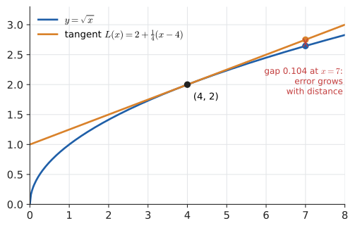
Take \(f(x) = \sqrt{x} = x^{1/2}\) and \(a = 4\). Try it: Estimate √4.1 with a tangent.
The true value is \(2.0248457\ldots\), so the error is about \(1.5\times 10^{-4}\). Check against the error estimate: \(f''(x) = -\tfrac{1}{4}x^{-3/2}\), so \(f''(4) = -\tfrac{1}{32}\), and \(\tfrac{1}{2}\cdot\tfrac{1}{32}\cdot(0.1)^2 \approx 1.56\times 10^{-4}\). The estimate also predicts the sign: since \(\sqrt{x}\) is concave down, the tangent lies above the curve and the approximation overshoots.
18.6.5. Worked example: small angles and the pendulum
Linearise \(\sin x\) at \(a = 0\): \(f(0) = 0\), \(f'(0) = \cos 0 = 1\), so \(L(x) = x\). For small angles in radians, \(\sin x \approx x\). At \(x = 0.1\) (about \(5.7^\circ\)), \(\sin 0.1 = 0.0998334\), an error under \(0.2\%\). Try it: sin x ≈ x, visually.
This is the step every Mechanics course takes with the simple pendulum. The exact equation of motion contains \(\sin\theta\); replacing it with \(\theta\) turns it into the equation of simple harmonic motion, whose solutions are sines and cosines with period \(2\pi\sqrt{\ell/g}\). That famous formula is only true for small swings — it is a linear approximation.
18.6.6. Worked example: error propagation with differentials
You measure a ball’s radius as \(10\) cm, with a possible error of \(\pm 0.1\) cm. How uncertain is the computed volume?
Relative to \(V = \tfrac{4}{3}\pi(1000) \approx 4189\ \text{cm}^3\), that is
A 1% error in the radius becomes a 3% error in the volume: cubing triples relative errors. (In general, for \(y = x^n\), relative error multiplies by \(n\).)
18.6.7. Where you’d use this
-
Finance: the rule of 70. How long does money take to double at 7% a year? Exactly, \(t = \ln 2/\ln 1.07 \approx 10.24\) years. The linearisation \(\ln(1 + r) \approx r\) gives \(t \approx 0.693/r\), which bankers round to "70 divided by the percentage": \(70/7 = 10\) years. The same shortcut tells you that 3% inflation halves the value of money in about 23 years.
-
Science and engineering. Error propagation (above) is how lab reports and engineering tolerances work; the small-angle approximation \(\sin\theta \approx \theta\) is used by surveyors and astronomers (an object 1 m wide seen at 1 km subtends about \(0.001\) rad), and by every pendulum clock.
-
Computing. Graphics and physics engines linearise constantly: a skinned character’s joints, a car’s suspension and a robot arm are simulated by replacing the nonlinear equations with their tangent-line versions for one small time step at a time. The extended Kalman filter in the sidebar below is the same move for navigation.
18.7. L’Hôpital’s rule
18.7.1. The problem
In Chapter 16 you met limits like \(\lim_{x\to 0}\frac{\sin x}{x}\), where plugging in gives \(\frac{0}{0}\) — an indeterminate form, meaning the answer depends on how fast numerator and denominator approach zero. Algebraic tricks and squeezing work sometimes. Is there a general tool? Yes: compare their rates of approach — their derivatives.
18.7.2. Why it works
Suppose \(f(a) = g(a) = 0\) and both are differentiable at \(a\) with \(g'(a) \ne 0\). Near \(a\), replace each by its linearisation:
Both functions start at zero; their ratio is governed by their speeds. The full theorem (proved with a generalisation of the Mean Value Theorem) states:
provided the right-hand limit exists (or is \(\pm\infty\)). It also works for \(a = \pm\infty\) and one-sided limits.
|
Indeterminate form
An indeterminate form is a limit shape whose value cannot be decided from the limits of the pieces alone: \(\frac{0}{0}\), \(\frac{\infty}{\infty}\), \(0\cdot\infty\), \(\infty - \infty\), \(0^0\), \(1^\infty\), \(\infty^0\). L’Hôpital applies directly only to the first two; the others are first rewritten as a quotient. |
18.7.3. Worked examples
1. \(\displaystyle\lim_{x\to 0}\frac{\sin x}{x}\): form \(\frac00\).
(Honesty note: the derivative of \(\sin x\) was itself derived using this limit in Chapter 17, so this is a consistency check, not an independent proof.)
2. \(\displaystyle\lim_{x\to 0}\frac{e^x - 1 - x}{x^2}\): form \(\frac00\). Apply twice:
3. \(\displaystyle\lim_{x\to\infty}\frac{\ln x}{x}\): form \(\frac{\infty}{\infty}\).
Logarithms grow more slowly than any line — the calculus behind "\(O(\log n)\) beats \(O(n)\)".
4. \(\displaystyle\lim_{x\to 0^+} x\ln x\): form \(0\cdot(-\infty)\). Rewrite as a quotient first:
This limit is why information theory can define \(0\log 0 = 0\) in the entropy formula.
|
When L’Hôpital does not apply
|
|
A theorem bought and paid for
The rule appeared in the first calculus textbook, Analyse des infiniment petits (1696), by the Marquis de l’Hôpital. But the mathematics was Johann Bernoulli’s: l’Hôpital had paid Bernoulli a salary for his discoveries, under an agreement that he could use them as he wished. Bernoulli’s letters, found in the 20th century, settled the matter. |
18.8. Taylor polynomials
18.8.1. The problem
A tangent line matches a function’s value and slope at one point. It is good nearby, and then drifts off. Could we do better by matching the bending too — the second derivative — and the third, and so on? And how do computers actually evaluate \(\sin x\), when the only operations a chip performs are addition and multiplication?
18.8.2. Intuition and why it works
Polynomials are the functions computers can evaluate with just \(+\) and \(\times\). So look for a polynomial
that agrees with \(f\) at \(x = 0\) in value and in its first \(n\) derivatives. Differentiate \(p\) repeatedly and set \(x = 0\); each time, every term vanishes except one:
The \(k!\) (k factorial, \(k! = 1\cdot 2\cdots k\), from Chapter 24 and Chapter 14) appears because differentiating \(x^k\) \(k\) times brings down \(k, k-1, \ldots, 1\). The result is the Taylor polynomial of degree \(n\) about \(0\) (also called a Maclaurin polynomial):
About a general centre \(a\), replace \(x\) by \((x - a)\) and evaluate derivatives at \(a\). Degree 1 is exactly the linearisation \(L(x)\).
|
Taylor polynomial
The degree-\(n\) Taylor polynomial of \(f\) about \(a\) is \(T_n(x) = \sum_{k=0}^{n}\frac{f^{(k)}(a)}{k!}(x - a)^k\), the unique polynomial of degree at most \(n\) matching \(f\) and its first \(n\) derivatives at \(a\). Notation: \(f^{(k)}\) is the \(k\)-th derivative (brackets distinguish it from a power), with \(f^{(0)} = f\). Letting \(n \to \infty\) gives the Taylor series. |
18.8.3. Worked example: \(\sin x \approx x - \frac{x^3}{6}\)
The derivatives of \(\sin x\) cycle with period 4: Try it: Add Taylor terms to sin x; Taylor series of sin x.
| \(k\) | \(f^{(k)}(x)\) | \(f^{(k)}(0)\) |
|---|---|---|
0 |
\(\sin x\) |
0 |
1 |
\(\cos x\) |
1 |
2 |
\(-\sin x\) |
0 |
3 |
\(-\cos x\) |
\(-1\) |
4 |
\(\sin x\) |
0 |
5 |
\(\cos x\) |
1 |
Substituting into the formula, the even terms vanish:
At \(x = 0.5\) (where \(\sin 0.5 = 0.4794255\ldots\)):
| Approximation | Value | Error |
|---|---|---|
\(x\) |
\(0.5\) |
\(2.1\times 10^{-2}\) |
\(x - x^3/6\) |
\(0.5 - 0.0208333 = 0.4791667\) |
\(2.6\times 10^{-4}\) |
\(x - x^3/6 + x^5/120\) |
\(0.4791667 + 0.0002604 = 0.4794271\) |
\(1.5\times 10^{-6}\) |
Each extra term gains about two decimal digits here. The same procedure gives the other two essential expansions:
(for \(e^x\), every derivative is \(e^x\), which is 1 at 0, so every coefficient is \(1/k!\)).
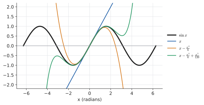
A short program shows the pattern — accuracy is excellent near the centre and poor far away:
import math

def sin_taylor(x, terms):
    """Sum the first `terms` nonzero terms of x - x^3/3! + x^5/5! - ..."""
    total, term = 0.0, x
    for k in range(terms):
        total += term
        term *= -x * x / ((2 * k + 2) * (2 * k + 3))
    return total

for x in (0.1, 0.5, 1.0, 3.0):
    row = [abs(sin_taylor(x, t) - math.sin(x)) for t in (1, 2, 3, 5)]
    print(f"x = {x:3}: " + "  ".join(f"{e:.1e}" for e in row))
x = 0.1: 1.7e-04 8.3e-08 2.0e-11 1.4e-17 x = 0.5: 2.1e-02 2.6e-04 1.5e-06 1.2e-11 x = 1.0: 1.6e-01 8.1e-03 2.0e-04 2.5e-08 x = 3.0: 2.9e+00 1.6e+00 3.8e-01 4.2e-03
Each new term is computed from the previous one (multiply by \(-x^2/((2k+2)(2k+3))\)), never from scratch — the factorials are never formed explicitly.
18.8.4. Where you’d use this
-
Physics: where \(\tfrac12 mv^2\) comes from. Einstein’s kinetic energy is \((\gamma - 1)mc^2\) with \(\gamma = (1 - v^2/c^2)^{-1/2}\). The degree-1 Taylor polynomial of \((1 - u)^{-1/2}\) is \(1 + \tfrac12 u\), so \(\gamma - 1 \approx \frac{v^2}{2c^2}\) and the kinetic energy is approximately \(\tfrac12 mv^2\), the Mechanics formula. At a tenth of the speed of light the two disagree by under 1% (\(\gamma - 1 = 0.005038\) against \(0.005\)). Try it: Linearise γ: ½mv².
-
Finance: bond risk. A bond’s price change for a small change \(\Delta y\) in interest rates is written as a Taylor polynomial: \(\frac{\Delta P}{P} \approx -D\,\Delta y + \tfrac12 C(\Delta y)^2\). The first-order coefficient \(D\) is the bond’s duration and the second-order one its convexity. A bond with duration 7 loses about 7% of its value when rates rise by one percentage point.
-
Computing. Beyond computing \(\sin\) (see the sidebar), second-order Taylor expansions are how optimisers such as Newton’s method model a loss function locally, and how game physics integrators are analysed for accuracy.
|
Know where you are
A Taylor polynomial is a local approximation. The table shows five terms of the sine series still miss by \(4\times 10^{-3}\) at \(x = 3\). And some functions' series only work in a limited range: the series of \(\ln(1 + x)\) converges only for \(-1 < x \le 1\), however many terms you take. Always use radians — the derivative of \(\sin x\) is \(\cos x\) only in radians. |
Try it: Where ln(1 + x) stops converging.
18.9. Exercises: rates, approximation, limits
-
(Recognition) Write down the linearisation of \(f(x) = e^x\) at \(a = 0\).
-
(Application) A stone dropped in a pond makes a circular ripple whose radius grows at 2 cm/s. How fast is the area growing when the radius is 10 cm?
-
(Application) Use a linear approximation to estimate \(\sqrt[3]{8.3}\) and \(\ln(1.05)\). Are your estimates too high or too low? Try it: Estimate ∛8.3 with a tangent.
-
(Application) Evaluate \(\displaystyle\lim_{x\to 0}\frac{1 - \cos x}{x^2}\) and \(\displaystyle\lim_{x\to\infty}\frac{x^2}{e^x}\).
-
(Problem solving) Use the degree-2 Taylor polynomial of \(e^x\) to estimate \(e^{0.1}\), and explain why \(1 - \cos x \approx x^2/2\) for small \(x\) agrees with your answer to question 4. Try it: e^0.1 from a Taylor polynomial.
Answers
-
\(f(0) = 1\), \(f'(0) = e^0 = 1\), so \(L(x) = 1 + x\).
-
\(A = \pi r^2\), so \(\frac{dA}{dt} = 2\pi r\frac{dr}{dt} = 2\pi(10)(2) = 40\pi \approx 125.7\ \text{cm}^2/\text{s}\).
-
\(f(x) = x^{1/3}\), \(a = 8\): \(f(8) = 2\), \(f'(x) = \tfrac13 x^{-2/3}\), \(f'(8) = \tfrac{1}{3\cdot 4} = \tfrac{1}{12}\). \(\sqrt[3]{8.3} \approx 2 + 0.3/12 = 2.025\) (true: \(2.02469\)). \(\ln\) at \(a = 1\): \(\ln 1 = 0\), derivative \(1/x = 1\), so \(\ln 1.05 \approx 0.05\) (true: \(0.04879\)). Both too high: both functions are concave down, so tangent lines lie above them.
-
First: form \(\frac00\); L’Hôpital gives \(\lim\frac{\sin x}{2x} = \frac12\lim\frac{\sin x}{x} = \frac12\). Second: form \(\frac\infty\infty\); twice gives \(\lim\frac{2x}{e^x} = \lim\frac{2}{e^x} = 0\).
-
\(e^{0.1} \approx 1 + 0.1 + 0.01/2 = 1.105\) (true: \(1.10517\)). From \(\cos x \approx 1 - x^2/2\), \(1 - \cos x \approx x^2/2\), so \(\frac{1 - \cos x}{x^2} \approx \frac12\) for small \(x\), matching the limit.
18.10. Newton’s method
This is the chapter’s centrepiece, and one of the most important algorithms in all of applied mathematics. We will build it in ten steps — what problem it solves, why that problem is hard, why a tangent line helps, how the formula falls out of the tangent, how to start, how to step, how to repeat, when to stop, when it works brilliantly, and when it fails — and only then hand it to Python.
18.10.1. 1. The problem: solve \(f(x) = 0\)
Many questions reduce to finding a root (or zero) of a function: a number \(r\) with \(f(r) = 0\).
-
What is \(\sqrt{2}\)? It is the positive root of \(f(x) = x^2 - 2\).
-
Where does \(\cos x\) equal \(x\)? At the root of \(f(x) = \cos x - x\).
-
Where is \(g\) maximised? At a root of \(f = g'\) (Section 18.3).
-
What interest rate makes a loan’s payments add up to its price? The root of a polynomial of high degree.
Any equation \(\text{left} = \text{right}\) can be rewritten as \(\text{left} - \text{right} = 0\), so "find a root" is the universal form of "solve an equation".
|
Root, zero, iteration
A root or zero of \(f\) is a value \(r\) with \(f(r) = 0\); graphically, where the curve crosses or touches the \(x\)-axis. An iterative method produces a sequence of approximations \(x_0, x_1, x_2, \ldots\) (read "x-nought, x-one, …"; the subscript is the step number), each computed from the previous one by the same rule. \(x_0\) is the initial guess. The method converges if \(x_n \to r\) as \(n \to \infty\) (a limit of a sequence, Chapter 14). |
18.10.2. 2. Why solving directly is often impossible
For linear and quadratic equations we have formulas (Chapter 5, Chapter 8). Cubics and quartics have formulas too, but they are monstrous. For polynomials of degree five and higher, the Abel–Ruffini theorem says there is no general formula in radicals at all. And equations that mix kinds of function, like \(\cos x = x\) or \(e^x = 3x\), typically have no closed-form solution in terms of familiar functions.
Yet these equations have perfectly definite answers, and we need them to 15 digits. The way forward is to stop looking for a formula for the answer, and instead look for a procedure that improves a guess.
18.10.3. 3. Why a tangent line helps
We cannot easily solve \(f(x) = 0\) for a curved \(f\). But we can trivially solve \(L(x) = 0\) for a straight line \(L\). And from Section 18.6 we know that near any point, a smooth curve is well approximated by its tangent line.
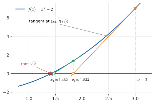
So: stand at your current guess \(x_n\) on the curve, at the point \((x_n, f(x_n))\). Draw the tangent there. Follow it down (or up) to where it crosses the \(x\)-axis. Because the tangent hugs the curve, the place where the tangent hits zero should be close to where the curve hits zero — closer than where you started. Take that crossing as the new guess and repeat.
18.10.4. 4. Deriving the formula from the tangent
The tangent at \(x_n\) has slope \(f'(x_n)\) and passes through \((x_n, f(x_n))\). In point-slope form:
Call its \(x\)-intercept \(x_{n+1}\). At that point \(y = 0\):
That is Newton’s method (also called the Newton–Raphson method):
Read it in words: the correction is the current height divided by the current slope. If you are at height \(f(x_n) = 6\) on a slope of \(6\), a straight line would reach zero after stepping back \(1\) unit. The minus sign points the step in the right direction automatically: positive height with positive slope means step left, and so on. Notice also the division by \(f'(x_n)\) in the third line — we have already spotted the method’s Achilles' heel.
18.10.5. 5. Choosing an initial value
Newton’s method needs a starting guess \(x_0\), and the quality of that guess matters more than for any other step. Good ways to get one:
-
Sketch or plot \(f\) and read off roughly where it crosses the axis.
-
Find a sign change. If \(f(a)\) and \(f(b)\) have opposite signs and \(f\) is continuous, there is a root between \(a\) and \(b\) (the Intermediate Value Theorem, Chapter 16). Start inside, near whichever end has the smaller \(|f|\).
-
Use the problem’s meaning. For \(\sqrt{2}\), anything between 1 and 2 is sensible; for a physical quantity, its order of magnitude is usually known.
-
Run a few steps of a safe method first (bisection, below), then switch to Newton.
Avoid starting near points where \(f'(x) = 0\) — turning points of the curve — for reasons we will see in step 10.
18.10.6. 6–7. Computing the next approximation, and repeating
Now do it by hand. Find \(\sqrt{2}\) using \(f(x) = x^2 - 2\), whose derivative is \(f'(x) = 2x\), starting from \(x_0 = 1\) (since \(1^2 = 1 < 2 < 4 = 2^2\), the root is between 1 and 2).
Substituting \(f\) and \(f'\) into the general formula first gives a specific iteration:
Iteration 1 (\(n = 0\)):
Iteration 2 (\(n = 1\)):
Iteration 3 (\(n = 2\)). Working in fractions keeps it exact:
Iteration 4 (\(n = 3\)):
Compare with the true value \(\sqrt{2} = 1.414\,213\,562\,373\,095\ldots\):
| \(n\) | \(x_n\) | error \(\lvert x_n - \sqrt2\rvert\) | correct digits |
|---|---|---|---|
0 |
1 |
\(4.1\times 10^{-1}\) |
0 |
1 |
1.5 |
\(8.6\times 10^{-2}\) |
1 |
2 |
1.416 666 666 666 7 |
\(2.5\times 10^{-3}\) |
3 |
3 |
1.414 215 686 274 5 |
\(2.1\times 10^{-6}\) |
6 |
4 |
1.414 213 562 374 7 |
\(1.6\times 10^{-12}\) |
12 |
Try it: Newton versus bisection for √2.
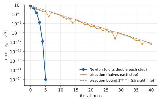
Look at the last column: 1, 3, 6, 12. The number of correct digits roughly doubles every step. Four steps of arithmetic you could do on paper give twelve correct digits.
18.10.7. 8. Deciding when to stop
An algorithm needs a termination condition. Since we don’t know the true root (if we did, we wouldn’t be computing it), we stop on evidence available inside the loop:
-
Step size: stop when \(|x_{n+1} - x_n| < \varepsilon\) for a chosen tolerance \(\varepsilon\) (epsilon, the conventional letter for "a small positive number"). With quadratic convergence, once the step is tiny the error is tinier still: the step from \(x_3\) to \(x_4\) above was \(2.1\times 10^{-6}\), while \(x_4\)'s actual error is about \(10^{-12}\).
-
Residual: stop when \(|f(x_n)| < \delta\). The residual \(f(x_n)\) measures how nearly the equation is satisfied. On its own it can mislead: if the curve is very flat, \(f(x)\) can be tiny far from the root.
-
Relative tolerance: for roots of large or unknown magnitude, use \(|x_{n+1} - x_n| < \varepsilon |x_{n+1}|\).
-
Iteration cap: always stop after some maximum number of steps and report failure. Newton’s method is not guaranteed to converge, and an unbounded loop is a bug.
Do not ask for more accuracy than the arithmetic can deliver. Double-precision floats carry about 16 significant digits (Chapter 32); a tolerance of \(10^{-20}\) on a root near 1 can never be met.
18.10.8. The procedure
Input: a function \(f(x)\), its derivative \(f'(x)\), an initial estimate \(x_0\), a tolerance \(\varepsilon\), and a maximum number of iterations.
Repeat for \(n = 0, 1, 2, \ldots\):
until
(If \(f'(x_n) = 0\), or the iteration cap is reached first, stop and report failure.)
Output: \(x_{n+1}\), an approximate root.
Try it: Step Newton’s cubic. ==== Worked example: Newton’s own cubic
Solve \(x^3 - 2x - 5 = 0\). This is the very equation Newton used to demonstrate his method around 1669; it has no rational root and one real root.
Set up. \(f(x) = x^3 - 2x - 5\), \(f'(x) = 3x^2 - 2\).
Initial value. Try integers: \(f(2) = 8 - 4 - 5 = -1\) and \(f(3) = 27 - 6 - 5 = 16\). The sign change puts a root between 2 and 3, and \(|f(2)|\) is much smaller, so take \(x_0 = 2\).
Iteration 1:
Iteration 2:
Iteration 3:
Iteration 4: \(f(x_3) \approx 1.74\times 10^{-9}\), \(f'(x_3) \approx 11.1614\), correction \(\approx 1.56\times 10^{-10}\), giving \(x_4 = 2.094\,551\,481\,542\,3\).
Stop? The last step was \(1.6\times 10^{-10}\); with \(\varepsilon = 10^{-8}\) we stop. The root is \(x \approx 2.094\,551\,48\). The corrections shrank \(0.1 \to 5.4\times 10^{-3} \to 1.7\times 10^{-5} \to 1.6\times 10^{-10}\) — again, the exponent roughly doubles.
18.10.9. Implementation in Python
The procedure translates almost line for line. We record every iterate so that we can study convergence.
def newton(f, df, x0, tol=1e-12, max_iter=50):
    """Return (root, history). Raises if it fails to converge."""
    x = x0
    history = [x]
    for _ in range(max_iter):
        fx, dfx = f(x), df(x)
        if dfx == 0:
            raise ZeroDivisionError(f"f'(x) = 0 at x = {x}; tangent is flat")
        x_new = x - fx / dfx
        history.append(x_new)
        if abs(x_new - x) < tol:
            return x_new, history
        x = x_new
    raise RuntimeError(f"no convergence after {max_iter} steps: {history[-3:]}")


root, hist = newton(lambda x: x**2 - 2, lambda x: 2 * x, 1.0)
for n, x in enumerate(hist):
    print(f"x_{n} = {x:.15f}   error = {abs(x - 2**0.5):.1e}")

root, hist = newton(lambda x: x**3 - 2*x - 5, lambda x: 3*x**2 - 2, 2.0)
print(root, len(hist) - 1, "steps")

try:
    newton(lambda x: x**3 - 2*x + 2, lambda x: 3*x**2 - 2, 0.0)
except RuntimeError as e:
    print(e)
x_0 = 1.000000000000000 error = 4.1e-01 x_1 = 1.500000000000000 error = 8.6e-02 x_2 = 1.416666666666667 error = 2.5e-03 x_3 = 1.414215686274510 error = 2.1e-06 x_4 = 1.414213562374690 error = 1.6e-12 x_5 = 1.414213562373095 error = 0.0e+00 x_6 = 1.414213562373095 error = 2.2e-16 2.0945514815423265 5 steps no convergence after 50 steps: [0.0, 1.0, 0.0]
Three things to notice. The hand calculation and the program agree digit for digit. After \(x_5\) the error is at the level of floating-point rounding — \(x_6\) differs from \(x_5\) by one unit in the last place, and that tiny step is what triggers the stop. And the last call, which we will explain shortly, never converges at all: the iteration cap turned an infinite loop into a clear error message.
18.10.10. 9. When Newton’s method works well: quadratic convergence
Why do the digits double? Let \(r\) be the root and write the error as \(e_n = x_n - r\). Expand \(f\) around \(x_n\) using a Taylor polynomial of degree 1 plus its error term (Section 18.8), evaluated at the root:
for some \(\xi\) between \(x_n\) and \(r\). Divide by \(f'(x_n)\) and rearrange:
The new error is proportional to the square of the old one. If the error is \(10^{-3}\), the next is about \(C\times 10^{-6}\), then \(C^3\times 10^{-12}\): the exponent doubles. This is quadratic convergence.
Check it on \(\sqrt2\): \(C \approx \frac{f''(r)}{2f'(r)} = \frac{2}{2\cdot 2\sqrt2} \approx 0.3536\). From \(e_3 = 2.124\times 10^{-6}\), the prediction is \(e_4 \approx 0.3536\times(2.124\times 10^{-6})^2 = 1.595\times 10^{-12}\), and the measured error was \(1.595\times 10^{-12}\).
The formula also explains what "works well" requires: \(f'(r) \ne 0\) (a simple root, so \(C\) is finite), \(f''\) not wild, and \(x_0\) close enough that \(|C e_0| < 1\). Under those conditions Newton’s method is the fastest practical root finder there is.
|
Order of convergence
A method has order of convergence \(p\) if \(|e_{n+1}| \approx C|e_n|^p\) for large \(n\). \(p = 1\) is linear convergence (a fixed number of digits gained per step — bisection gains one binary digit); \(p = 2\) is quadratic (digits double — Newton at a simple root). The secant method has \(p = \tfrac{1+\sqrt5}{2} \approx 1.618\), the golden ratio. |
Try it: Race the two methods.
18.10.11. 10. When Newton’s method fails
Quadratic convergence is a local promise: it holds once you are close enough. Far from a root, or at a badly behaved one, the tangent line is a poor model of the curve, and following it can lead anywhere. These are not curiosities; you will meet every one of them in practice.
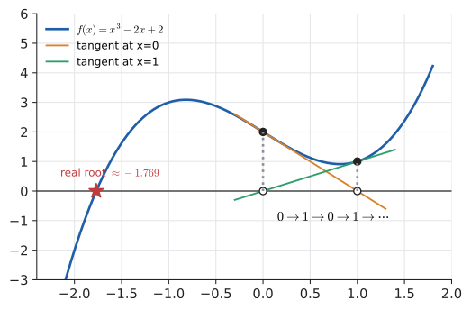
Oscillation: \(f(x) = x^3 - 2x + 2\) from \(x_0 = 0\). Here \(f'(x) = 3x^2 - 2\). Try it: Watch the 0–1 cycle.
We are back where we started; the iteration cycles \(0, 1, 0, 1, \ldots\) forever. Worse, the cycle attracts nearby starts: from \(x_0 = 0.1\) the iterates are drawn into the same 0–1 cycle. The only real root is near \(-1.769\), on the other side of a hump. Start at \(x_0 = -2\) instead and Newton gives \(-1.8,\ -1.76995,\ -1.7692927,\ -1.769292354\) — converged in four steps.
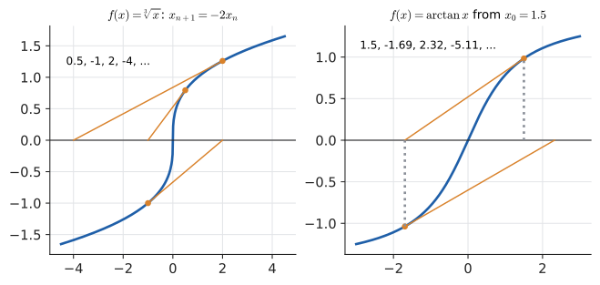
Divergence: the iterates run away. For \(f(x) = \sqrt[3]{x} = x^{1/3}\) (root at 0), \(f'(x) = \tfrac13 x^{-2/3}\), and Try it: Find the arctan threshold; Newton diverging on ∛x.
Every step doubles the distance from the root, from any nonzero start: \(0.5, -1, 2, -4, \ldots\). The curve is so steep at its root (vertical tangent) that the tangents from elsewhere overshoot. A less contrived example: \(f(x) = \arctan x\) from \(x_0 = 1.5\) gives \(-1.694,\ 2.321,\ -5.114,\ 32.30,\ -1575.3, \ldots\) — the curve flattens out away from the root, so each tangent shoots further. (From \(x_0 = 1\) it converges; the boundary is near \(x_0 \approx 1.39\).)
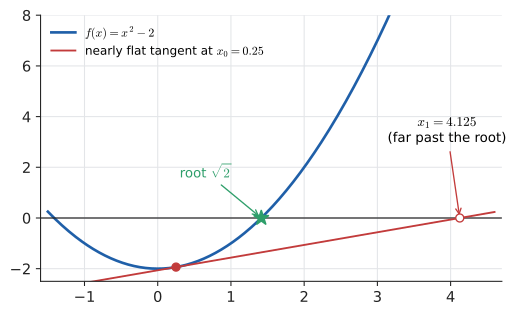
Flat tangent: \(f'(x_n) \approx 0\). The correction \(f(x_n)/f'(x_n)\) divides by the slope; near a turning point the slope is tiny and the step is huge. For \(x^2 - 2\) from \(x_0 = 0.01\): Try it: The flat-tangent leap.
Here the parabola is kind and the iterates crawl back (\(50.01, 25.03, 12.55, 6.36, 3.34, 1.97, 1.49, 1.416, \ldots\)), costing 11 steps instead of 5. On a function with several roots the giant leap usually lands near a different root, or somewhere the method then diverges. Exactly at \(f'(x_n) = 0\) the tangent is horizontal, never meets the axis, and the formula divides by zero.
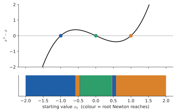
Wrong root, and sensitive dependence on \(x_0\). \(f(x) = x^3 - x = x(x-1)(x+1)\) has roots \(-1, 0, 1\). You might expect Newton to find the nearest one. Not so: starting from \(0.44\) reaches \(0\); from \(0.45\) it reaches \(-1\); from \(0.46\) it reaches \(+1\); from \(0.5\) it reaches \(-1\) again. Near \(x = \pm 1/\sqrt{3} \approx \pm 0.577\), where \(f' = 0\), tiny tangents throw the iterate across the graph. The set of starting values that lead to a given root is that root’s basin of attraction, and the basins interleave in ever finer bands near \(\pm 1/\sqrt5 \approx \pm 0.447\). Try it: Zoom into the basins.
Slow convergence at a repeated root. For \(f(x) = (x - 1)^2\), the root \(x = 1\) is a double root where \(f'(1) = 0\) too. The iteration becomes \(x_{n+1} = x_n - \frac{(x_n - 1)^2}{2(x_n - 1)} = x_n - \frac{x_n - 1}{2}\): the error merely halves each step. Newton degrades to linear convergence — no better than bisection — whenever the curve touches the axis instead of crossing it. Try it: Newton at a double root.
|
Newton’s method: checklist of failure modes
Defences: plot first; bracket the root with a sign change; cap the iterations; reject steps that leave the bracket and fall back to bisection (that is what robust library routines do); check the final residual \(|f(x)|\). |
18.10.12. Alternatives and choosing a method
Newton’s method is one of several ways to solve \(f(x) = 0\). The most important companion is bisection.
Bisection. If \(f(a)\) and \(f(b)\) have opposite signs, a root lies in \(\left[a, b\right]\). Evaluate the midpoint \(m = \frac{a+b}{2}\); whichever half still has a sign change contains a root; keep that half and repeat.
def bisection(f, a, b, tol=1e-12):
    fa = f(a)
    if fa * f(b) > 0:
        raise ValueError("f(a) and f(b) must have opposite signs")
    steps = 0
    while b - a > tol:
        m = (a + b) / 2
        fm = f(m)
        if fa * fm <= 0:
            b = m
        else:
            a, fa = m, fm
        steps += 1
    return (a + b) / 2, steps


print(bisection(lambda x: x**2 - 2, 1.0, 2.0))
(1.414213562372879, 40)
Forty steps for twelve digits, against Newton’s four or five. But bisection cannot fail once you have a bracket: the interval halves every time, so after \(n\) steps the error is at most \((b - a)/2^{n}\). It is binary search (Chapter 12) applied to a continuous function.
Secant method. Replace \(f'(x_n)\) by the slope of the secant through the last two iterates: \(x_{n+1} = x_n - f(x_n)\dfrac{x_n - x_{n-1}}{f(x_n) - f(x_{n-1})}\). No derivative needed; order \(\approx 1.618\); same failure modes as Newton.
Closed-form algebra. If a formula exists, use it. \(x^2 - 5x + 6 = 0\) practically begs to be factored as \((x - 2)(x - 3) = 0\); running Newton’s method on it would be rather silly.
| Method | Needs | Speed | Reliability |
|---|---|---|---|
Algebra / formula |
a solvable form |
instant, exact |
perfect, when available |
Bisection |
continuous \(f\), a sign-change bracket |
linear: 1 bit per step (~3.3 steps per decimal digit) |
guaranteed once bracketed |
Newton |
\(f\) and \(f'\), a good \(x_0\) |
quadratic: digits double |
can diverge, cycle, or jump roots |
Secant |
\(f\), two starting points |
order ~1.6, no derivative cost |
like Newton |
Hybrid (e.g. Brent’s method) |
a bracket |
near-Newton speed |
guaranteed |
Choosing: use algebra when it applies. When it doesn’t: if you have a good starting guess and a cheap derivative (or need to solve many similar equations — e.g. a square root for every pixel), use Newton. If you know nothing about where the root is, or reliability matters more than speed, bracket and bisect. In production code, use a hybrid: library routines such as Brent’s method take a fast Newton- or secant-like step when it stays inside the bracket and a bisection step when it doesn’t, getting both speed and a guarantee. Understanding the two pure methods is how you understand — and debug — the hybrid.
18.10.13. Where you’d use this
-
Square roots, division and reciprocals in hardware and software. Calculators and CPUs compute \(\sqrt{a}\) and \(1/a\) by Newton iterations from a table-lookup first guess.
-
Finance: internal rate of return. You invest £1000 and receive £400 at the end of each of the next three years. The internal rate of return is the interest rate \(r\) at which those payments are worth exactly £1000 today: \(f(r) = \frac{400}{1+r} + \frac{400}{(1+r)^2} + \frac{400}{(1+r)^3} - 1000 = 0\), a cubic in \(1/(1+r)\). Newton from \(r_0 = 0.1\) gives \(r_1 = 0.096997\), \(r_2 = 0.0970103\): an IRR of about 9.70%. Spreadsheet
IRRfunctions do exactly this — and print an error when the iteration fails to converge. -
Engineering and physics: implicit time-stepping in simulations solves a nonlinear equation at every step, by Newton’s method.
-
Optimisation: applied to \(g'(x) = 0\), Newton’s method finds stationary points: \(x_{n+1} = x_n - g'(x_n)/g''(x_n)\). Its many-variable form uses the matrix of second derivatives (Chapter 20).
-
Graphics and geometry: ray tracers find where a ray hits a curved surface by solving \(f(t) = 0\) along the ray.
|
Older than Newton, named after Newton
For \(f(x) = x^2 - a\), Newton’s formula simplifies to \(x_{n+1} = \tfrac12\left(x_n + \tfrac{a}{x_n}\right)\): average your guess with \(a\) divided by your guess. This is the Babylonian (or Heron’s) method, and a Babylonian clay tablet, YBC 7289 (around 1700 BCE), records \(\sqrt2 \approx 1.414\,213\) in base 60 — accurate to about one part in a million. Newton (around 1669) described his method on the cubic \(x^3 - 2x - 5 = 0\) as a sequence of polynomial substitutions, without derivatives; Joseph Raphson published the simpler iterative form in 1690; and the tangent-line formula we use came later still, with Thomas Simpson in 1740. |
|
Newton’s method explorer
Adjust the starting value \(x_0\) for Newton’s method with a slider and observe which root it reaches. The curve is drawn with each tangent line and each new iterate animated, and a side panel shows a table of \(x_n\), \(f(x_n)\), \(f'(x_n)\) and the correction. Preset functions: \(x^2 - 2\) (calm), \(x^3 - 2x + 2\) (find the start that cycles), \(\arctan x\) (find the divergence threshold near 1.39), and \(x^3 - x\) (colour the starting line by which root wins and zoom into the interleaved basins). Toggle "bisection" to race the two methods on the same function and plot their errors on a log scale. Extension: in the complex plane (Chapter 15), colour each starting point \(z_0\) by the root of \(z^3 - 1\) it reaches, and watch a fractal appear. |
18.11. A teaser: gradient descent
Newton’s method finds where \(f(x) = 0\). Optimisation needs where \(g'(x) = 0\). A more modest cousin of Newton’s method does this without second derivatives, and it is the engine of modern machine learning.
Idea. To minimise \(g\), stand at \(x_n\) and look at the slope. If \(g'(x_n) > 0\), downhill is to the left; if \(g'(x_n) < 0\), downhill is to the right. So step against the slope, by an amount proportional to it:
where \(\eta\) (eta) is a small positive step size, called the learning rate in machine learning. Steep slope: big step. Flat ground (near a minimum): small steps.
Example. Minimise \(g(x) = (x - 3)^2 + 1\), with \(g'(x) = 2(x - 3)\), from \(x_0 = 0\) with \(\eta = 0.2\): Try it: Step down the parabola.
def gradient_descent(df, x0, eta=0.2, steps=8):
    x = x0
    for n in range(steps):
        x = x - eta * df(x)
        print(f"step {n + 1}: x = {x:.4f}")
    return x

gradient_descent(lambda x: 2 * (x - 3), 0.0)
step 1: x = 1.2000 step 2: x = 1.9200 step 3: x = 2.3520 step 4: x = 2.6112 step 5: x = 2.7667 step 6: x = 2.8600 step 7: x = 2.9160 step 8: x = 2.9496
The distance to the minimum at 3 is multiplied by \(1 - 2\eta = 0.6\) each step: linear convergence, much slower than Newton. (Newton on \(g'\), namely \(x - g'(x)/g''(x) = x - (x - 3) = 3\), lands on the minimum in one step, because it uses the curvature \(g''\) to choose the step.) Too large an \(\eta\) — try \(\eta = 1.1\) — and the iterates overshoot and diverge, the gradient-descent cousin of Newton’s failure modes. Try it: Watch η = 1.1 diverge.
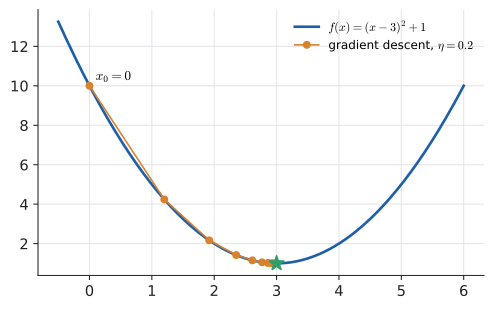
Why use the slower method? Because with a million parameters, the "second derivative" becomes a million-by-million matrix, too big to form, let alone invert; the first derivatives (the gradient, Chapter 20) can be computed for the cost of a few evaluations of the function by automatic differentiation (Chapter 17). Training a neural network is gradient descent, with clever choices of \(\eta\), on a function of millions of variables (Chapter 33).
18.12. Exercises: Newton’s method
-
(Recognition) Write down the Newton iteration for \(f(x) = x^3 - 10\), and simplify it.
-
(Application) Starting from \(x_0 = 2\), perform three Newton iterations for \(\sqrt[3]{10}\), showing \(f(x_n)\), \(f'(x_n)\) and the correction at each step.
-
(Application) Solve \(\cos x = x\) with Newton’s method from \(x_0 = 1\). Give \(x_1\) and \(x_2\) with all intermediate values.
-
(Problem solving) Explain, with a sketch, why Newton’s method for \(f(x) = x^3 - 2x + 2\) from \(x_0 = 0.5\) wanders before converging (iterates: \(1.4, 0.899, -1.289, -2.106, -1.829, -1.772, \ldots\)). Where is \(f'(x) = 0\)?
-
(Problem solving) For \(f(x) = x^2 - a\) (\(a > 0\)) show that Newton’s method is the Babylonian rule \(x_{n+1} = \tfrac12(x_n + a/x_n)\), and that from any \(x_0 > 0\) the iterates after the first are all \(\ge \sqrt{a}\). (Hint: \(x_{n+1} - \sqrt a = (x_n - \sqrt a)^2/(2x_n)\).)
-
(Problem solving) You need to solve \(e^x = 3x\) in a program that runs a million times per second, and also once in a one-off script. Which method would you choose in each case and why?
Answers
-
\(f'(x) = 3x^2\), so \(x_{n+1} = x_n - \frac{x_n^3 - 10}{3x_n^2} = \frac{2x_n^3 + 10}{3x_n^2} = \frac{2}{3}x_n + \frac{10}{3x_n^2}\).
-
\(n=0\): \(f(2) = 8 - 10 = -2\), \(f'(2) = 12\), correction \(-2/12 = -0.16667\), \(x_1 = 2.16667\). \(n=1\): \(f(x_1) = 10.17130 - 10 = 0.17130\), \(f'(x_1) = 14.08333\), correction \(0.012163\), \(x_2 = 2.15450\). \(n=2\): \(f(x_2) = 0.000960\), \(f'(x_2) = 13.92566\), correction \(0.0000689\), \(x_3 = 2.1544347\). (True: \(2.15443469\ldots\).)
-
\(f(x) = \cos x - x\), \(f'(x) = -\sin x - 1\). \(n=0\): \(f(1) = 0.540302 - 1 = -0.459698\), \(f'(1) = -0.841471 - 1 = -1.841471\), correction \(-0.459698/-1.841471 = 0.249636\), \(x_1 = 1 - 0.249636 = 0.750364\). \(n=1\): \(f(x_1) = 0.731440 - 0.750364 = -0.018923\), \(f'(x_1) = -0.681905 - 1 = -1.681905\), correction \(0.011251\), \(x_2 = 0.739113\). Converges to \(0.7390851\).
-
\(f'(x) = 3x^2 - 2 = 0\) at \(x = \pm\sqrt{2/3} \approx \pm 0.816\). Starting at 0.5 the curve is near its local minimum at \(0.816\), where the tangent is shallow; the tangent at 0.5 (slope \(-1.25\)) sends the iterate right to 1.4, then the iterate at 0.899 is close to the turning point and its shallow tangent throws it far left, past the root, to \(-1.289\). From there on it is on the steep left branch and converges quickly to \(-1.7693\).
-
\(x_{n+1} = x_n - \frac{x_n^2 - a}{2x_n} = \frac{2x_n^2 - x_n^2 + a}{2x_n} = \frac{x_n^2 + a}{2x_n} = \frac12\left(x_n + \frac{a}{x_n}\right)\). Then \(x_{n+1} - \sqrt a = \frac{x_n^2 - 2\sqrt a\, x_n + a}{2x_n} = \frac{(x_n - \sqrt a)^2}{2x_n} \ge 0\) for \(x_n > 0\). So every iterate after \(x_0\) is at or above \(\sqrt a\), and (being above) each further step moves down toward it — no failure is possible for \(x_0 > 0\).
-
Graph first: \(e^x - 3x\) has two roots (near 0.62 and 1.51), because \(f(0) = 1 > 0\), \(f(1) = e - 3 < 0\), \(f(2) = e^2 - 6 > 0\). For the high-volume program: Newton (\(f'(x) = e^x - 3\) is cheap) from a fixed good starting value inside the right bracket, with a cap and a fallback — e.g. from \(x_0 = 0.5\): \(0.6100, 0.6190, \ldots\). Avoid starting near \(x = \ln 3 \approx 1.099\), where \(f' = 0\). For the one-off script, robustness beats speed: bisection on \(\left[0,1\right]\) (or a library hybrid such as Brent’s method) is simplest to get right.
18.13. Interactive tools
Browser tools on the companion website that go with this chapter. Each example link in the chapter opens one of them with that example already set up.
18.14. Mastery check
-
Find and classify the stationary points of \(f(x) = 2x^3 - 3x^2 - 12x + 1\), and give its inflection point.
-
An open-topped box with a square base must hold \(32\,000\ \text{cm}^3\). Find the dimensions that use the least material.
-
Use a linear approximation to estimate \((1.02)^{10}\). Is the estimate high or low?
-
Evaluate \(\displaystyle\lim_{x\to 0}\frac{e^{2x} - 1}{x}\).
-
Write the degree-3 Taylor polynomial of \(\sin x\) about 0 and use it to estimate \(\sin 0.2\).
-
Derive Newton’s formula from the tangent line, then perform two iterations for \(f(x) = x^2 - 5\) from \(x_0 = 2\).
-
Newton’s method on \(x^3 - 2x + 2\) from \(x_0 = 0\) does not converge. Show what happens in two steps, and suggest two different fixes.
Decision rule: All correct without hesitation → move on to Chapter 19. Stuck on 1–2 → reread Section 18.1; on 2 → Section 18.3; on 3–5 → Section 18.6, Section 18.7 and Section 18.8; on 6–7 → Section 18.10 and Section 18.10.11. Stuck on more → work the section exercises first.
Mastery check answers
-
\(f'(x) = 6x^2 - 6x - 12 = 6(x - 2)(x + 1)\): stationary at \(x = -1\) and \(x = 2\). \(f''(x) = 12x - 6\). \(f''(-1) = -18 < 0\): local max \(f(-1) = -2 - 3 + 12 + 1 = 8\). \(f''(2) = 18 > 0\): local min \(f(2) = 16 - 12 - 24 + 1 = -19\). Inflection where \(12x - 6 = 0\): \(x = \tfrac12\), \(f(\tfrac12) = \tfrac14 - \tfrac34 - 6 + 1 = -5.5\).
-
Base side \(x\), height \(h\); constraint \(x^2 h = 32\,000\), so \(h = 32\,000/x^2\). Material \(S = x^2 + 4xh = x^2 + 128\,000/x\). \(S'(x) = 2x - 128\,000/x^2 = 0 \Rightarrow x^3 = 64\,000 \Rightarrow x = 40\). \(S''(x) = 2 + 256\,000/x^3 > 0\): minimum. \(h = 32\,000/1600 = 20\). Box \(40 \times 40 \times 20\) cm, using \(4800\ \text{cm}^2\).
-
\(f(x) = x^{10}\) at \(a = 1\): \(f(1) = 1\), \(f'(1) = 10\), so \((1.02)^{10} \approx 1 + 10(0.02) = 1.2\). True value \(1.21899\): the estimate is low, because \(x^{10}\) is concave up there (tangent below the curve).
-
Form \(\frac00\). L’Hôpital: \(\lim_{x\to 0}\frac{2e^{2x}}{1} = 2\). (Or: \(e^{2x} \approx 1 + 2x\), so the ratio \(\approx 2x/x = 2\).)
-
\(T_3(x) = x - \frac{x^3}{6}\). \(\sin 0.2 \approx 0.2 - \frac{0.008}{6} = 0.2 - 0.001\,333 = 0.198\,667\) (true: \(0.198\,669\)).
-
Tangent at \(x_n\): \(y = f(x_n) + f'(x_n)(x - x_n)\); setting \(y = 0\) gives \(x_{n+1} = x_n - f(x_n)/f'(x_n)\). With \(f'(x) = 2x\): \(n=0\): \(f(2) = -1\), \(f'(2) = 4\), \(x_1 = 2 + 0.25 = 2.25\). \(n=1\): \(f(2.25) = 5.0625 - 5 = 0.0625\), \(f'(2.25) = 4.5\), correction \(0.013\,889\), \(x_2 = 2.236\,111\) (true \(\sqrt5 = 2.236\,068\)).
-
\(x_1 = 0 - \frac{2}{-2} = 1\); \(x_2 = 1 - \frac{1}{1} = 0\): a 2-cycle. Fixes: (a) choose a better \(x_0\) from a sketch or sign change — \(f(-2) = -2 < 0 < 2 = f(0)\), so start at \(x_0 = -2\), which converges to \(-1.76929\) in four steps; (b) use bisection on \(\left[-2, 0\right]\) (or a bracketed hybrid), which cannot cycle.