Volume 2: Continuous Mathematics · Part V: Calculus
Chapter 16. Limits and Continuity
Chapter map: calculus rests on one idea — the limit — which makes precise what it means for a quantity to "approach" a value. This chapter starts from a concrete puzzle (what does "travelling at 63 mph at this instant" mean?), builds the informal idea of a limit with tables and pictures, then develops the tools for computing limits, the notion of continuity, the intermediate value theorem with its algorithmic twin the bisection method, and limits at infinity. An optional section presents the rigorous ε–δ definition as a game. Throughout, we watch what happens when a computer tries to take limits with floating-point numbers.
Why this chapter matters: a speed camera, a fitness tracker’s live pace, the temperature your coffee settles to, the rate of return on an investment, and the claim that one sorting algorithm beats another "for large inputs" are all limits. So is every derivative and integral in the rest of the book. And because computers cannot take limits exactly, the same idea explains a whole family of numerical bugs.
16.1. The problem: speed at an instant
16.1.1. What does "63 mph right now" mean?
Average speed is easy. If a car covers 120 miles in 2 hours, its average speed is
where \(\Delta\) (capital Greek delta) means "change in". But a speedometer claims something stronger: at precisely this instant, the car is travelling at 63 mph. What can that mean? At a single instant the car travels zero distance in zero time, and \(\frac{0}{0}\) is meaningless. Yet the speedometer reading is clearly not nonsense — a police radar gun and the car agree on it, and physics depends on it.
Here is a concrete version. A car accelerates steadily so that, \(t\) hours after setting off, it has travelled
How fast is it going at \(t = 1.5\) hours?
16.1.2. Shrink the interval
We cannot compute speed over an interval of zero length, but we can compute average speed over short intervals from \(t = 1.5\) to \(t = 1.5 + h\), and watch what happens as \(h\) shrinks: Try it: Watch the secants shrink.
def d(t):
    """Distance travelled (miles) after t hours."""
    return 21 * t**2

t0 = 1.5
for h in [1, 0.5, 0.1, 0.01, 0.001, 0.0001]:
    avg = (d(t0 + h) - d(t0)) / h
    print(f"h = {h:<7} average speed = {avg:.6f} mph")
h = 1 average speed = 84.000000 mph h = 0.5 average speed = 73.500000 mph h = 0.1 average speed = 65.100000 mph h = 0.01 average speed = 63.210000 mph h = 0.001 average speed = 63.021000 mph h = 0.0001 average speed = 63.002100 mph
The averages are homing in on 63. No single interval gives exactly 63 — every one gives a bit more, because the car is speeding up during the interval — but by making \(h\) small enough we can get as close to 63 as we like. So we define the instantaneous speed to be 63 mph: the value the average speeds approach as the interval shrinks to nothing.
Algebra confirms the table and shows exactly why:
For every nonzero \(h\), the average speed is \(63 + 21h\). As \(h\) gets closer to 0, this gets closer to 63. We never set \(h = 0\) (the original fraction would be \(\frac00\)); we ask what the expression approaches.
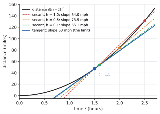
On the distance–time graph, each average speed is the slope of a secant line through two points of the curve. As the second point slides towards the first, the secants pivot towards the tangent line, which just touches the curve at \(t = 1.5\). Its slope is the instantaneous speed. This is the derivative, and it is the subject of Chapter 17. Before we can do that properly, we need to understand the process at its heart: the limit.
|
Secant to tangent
Show the graph of \(d(t) = 21t^2\) with a fixed point at \(t = 1.5\) and a draggable second point. Display the secant line, its slope, and \(h\). As the user drags the second point in from either side, a table records the slopes, and the secant visibly rotates into the tangent. Let the user change \(d(t)\) to \(\sqrt t\), \(\sin t\), or \(|t - 1.5|\) (where the left and right secants disagree). |
16.1.3. Where you’d use this
-
Speed cameras (everyday): UK average-speed cameras photograph your number plate at two points and divide distance by time. Covering a 2 km section in 1 minute 20 seconds means \(2 / (80/3600) = 90\) km/h, even if you briefly hit 110 km/h in the middle. A police radar or laser gun instead measures over a few milliseconds, effectively a very small \(h\). The radar is approximating the limit. The average-speed camera deliberately doesn’t.
-
Sport and fitness: a running watch shows your "current pace" from GPS positions a second or two apart, which is a secant over a short interval. Make the interval too short and GPS jitter (a few metres of error) swamps the real movement, so the reading jumps about. That is the same trade-off between a small \(h\) and noise that Section 16.11 finds in floating-point arithmetic.
-
Physics and computing: every physics engine in a game advances positions using velocities, that is, instantaneous rates, over small time steps \(\Delta t\) (often \(1/60\) s). The smaller the step, the closer the simulation is to the limit, and the more it costs to run.
16.2. The idea of a limit
16.2.1. Intuition
The pattern is general. We have a function \(f\) and a point \(a\), and we want to know what value \(f(x)\) approaches as \(x\) gets closer and closer to \(a\) — often precisely because we cannot (or do not want to) evaluate \(f(a)\) itself.
|
Limit (informal)
We write
\[\lim_{x \to a} f(x) = L\]
and say "the limit of \(f(x)\) as \(x\) approaches (or tends to) \(a\) is \(L\)" if \(f(x)\) can be made as close to \(L\) as we like by taking \(x\) sufficiently close to \(a\), but not equal to \(a\). Reading the notation piece by piece: lim abbreviates "limit"; the subscript \(x \to a\) says which variable is moving and where it is heading; \(f(x)\) is the expression being watched; \(L\) is the value it approaches. An alternative notation is \(f(x) \to L \text{ as } x \to a\). |
Two features of the definition are crucial.
-
\(x\) never equals \(a\). The limit is about the behaviour of \(f\) near \(a\), not at \(a\). The value \(f(a)\) may be different from the limit, or not exist at all.
-
\(x\) approaches from both sides. Unless stated otherwise, \(x\) may approach \(a\) from the left (values less than \(a\)) or from the right, and \(f(x)\) must approach the same \(L\) either way.
16.2.2. A function with a hole
Consider Try it: Explore the hole at 2.
At \(x = 2\) this is \(\frac00\): undefined. But a table of values near 2 tells a clear story:
| \(x\) | 1.9 | 1.99 | 1.999 | 2.001 | 2.01 | 2.1 |
|---|---|---|---|---|---|---|
\(f(x)\) |
3.9 |
3.99 |
3.999 |
4.001 |
4.01 |
4.1 |
From both sides, \(f(x)\) approaches 4. The algebra explains it: for \(x \ne 2\),
so the graph is the line \(y = x + 2\) with a single point missing at \((2, 4)\). Therefore \(\lim_{x\to2} f(x) = 4\), even though \(f(2)\) does not exist.
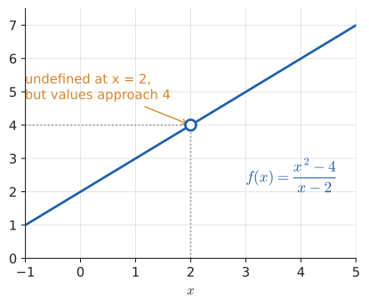
This is exactly the situation of the car: the average-speed formula \(\frac{d(1.5 + h) - d(1.5)}{h}\) is undefined at \(h = 0\), but equals \(63 + 21h\) everywhere else, so its limit as \(h \to 0\) is 63. Every derivative is a limit of this "0/0" type. That is why limits come first.
|
Tables of values can lie
A table suggests a limit; it does not prove one. Consider \(g(x) = \sin(\pi/x)\) as \(x \to 0\). At \(x = 0.1, 0.01, 0.001, \ldots\) we get \(\sin(10\pi), \sin(100\pi), \sin(1000\pi), \ldots\), all exactly 0. The table screams "the limit is 0". But at \(x = \frac{2}{5}, \frac{2}{9}, \frac{2}{13}, \ldots\) (which also approach 0), \(g(x) = \sin(\frac{5\pi}{2}), \sin(\frac{9\pi}{2}), \ldots = 1\). The function oscillates between \(-1\) and 1 infinitely often near 0, and has no limit. Tables sample; algebra and reasoning decide. Use tables to form a conjecture, then confirm it. |
Try it: See a table lie.
16.3. One-sided limits, and limits that do not exist
16.3.1. One-sided limits
Sometimes a function behaves differently on the two sides of a point. The sign function \(\frac{|x|}{x}\) equals \(-1\) for every negative \(x\) and \(+1\) for every positive \(x\) (and is undefined at 0). Try it: One-sided limits of |x|/x.
|
One-sided limits
\(\lim_{x\to a^-} f(x) = L\) (the left-hand limit) means \(f(x)\) approaches \(L\) as \(x\) approaches \(a\) from below (\(x < a\)). \(\lim_{x\to a^{+}} f(x) = L\) (the right-hand limit) means the same with \(x > a\). The superscript \(-\) or \({+}\) is a direction, not a sign on \(a\): \(x \to 2^-\) means \(x\) increases towards 2 through values like 1.9, 1.99, … Key fact: the two-sided limit \(\lim_{x \to a} f(x)\) exists and equals \(L\) exactly when both one-sided limits exist and both equal \(L\). |
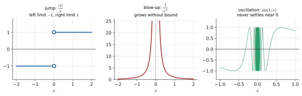
For the sign function, \(\lim_{x\to0^-} \frac{|x|}{x} = -1\) and \(\lim_{x\to0^{+}}\frac{|x|}{x} = 1\). They disagree, so \(\lim_{x\to0}\frac{|x|}{x}\) does not exist.
One-sided limits also handle edges of domains: \(\sqrt x\) is only defined for \(x \ge 0\), and \(\lim_{x\to0^{+}}\sqrt x = 0\) is the only sensible question to ask at 0.
16.3.2. Three ways for a limit to fail
-
Jump. The one-sided limits exist but differ, as for \(\frac{|x|}{x}\) at 0, or the floor function \(\lfloor x \rfloor\) (round down) at any integer. Try it: Watch 1/x² blow up; Watch sin(1/x) oscillate.
-
Blow-up. \(f(x)\) grows without bound. As \(x \to 0\), \(\frac{1}{x^2}\) exceeds every number you name. We write \(\lim_{x\to0}\frac{1}{x^2} = \infty\) — but this is a description of how the limit fails, not a number. For \(\frac1x\), the two sides go opposite ways: \(\lim_{x\to0^{+}}\frac1x = +\infty\), \(\lim_{x\to0^-}\frac1x = -\infty\).
-
Oscillation. \(\sin(1/x)\) swings between \(-1\) and 1 infinitely often in every interval around 0, never settling.
|
Infinite limit
\(\lim_{x \to a} f(x) = \infty\) means \(f(x)\) becomes larger than any given number when \(x\) is close enough to \(a\) (\(x \ne a\)). Similarly for \(-\infty\). The limit does not exist as a real number; the notation records the direction of failure. The line \(x = a\) is then a vertical asymptote of the graph. |
16.4. Limit laws and direct substitution
16.4.1. The problem
Tables are slow and unreliable. We want rules that compute limits of complicated expressions from limits of simple ones.
16.4.2. The laws
Suppose \(\lim_{x\to a} f(x) = L\) and \(\lim_{x\to a} g(x) = M\) both exist, and \(c\) is a constant. Then:
together with the two basic limits \(\lim_{x\to a} c = c\) and \(\lim_{x\to a} x = a\).
These are intuitive — if \(f\) is near \(L\) and \(g\) is near \(M\), then \(f + g\) is near \(L + M\) — and they can be proved from the formal definition in Section 16.10. The essential condition is in the first line: both limits must exist. The quotient law has a second condition: the denominator’s limit must not be zero. Almost every interesting limit violates that second condition, which is why we need techniques.
16.4.3. Direct substitution
Applying the laws repeatedly to a polynomial gives \(\lim_{x\to a} p(x) = p(a)\): just substitute. The same holds for a rational function \(\frac{p(x)}{q(x)}\) whenever \(q(a) \ne 0\), and, as we will see under continuity, for every "standard" function (roots, exponentials, logarithms, sine, cosine) at points of its domain.
Worked example. \(\lim_{x\to3}\dfrac{x^2 + 2x}{x - 1}\).
Always try substitution first. If it gives a number, you are done. If it gives \(\frac{c}{0}\) with \(c \ne 0\), the function blows up (examine the signs on each side). If it gives \(\frac{0}{0}\), you have an indeterminate form — the answer could be anything, and you need to do more work.
|
Indeterminate form
An indeterminate form is a limit whose naive substitution gives an expression like \(\frac00\), \(\frac{\infty}{\infty}\), \(\infty - \infty\), \(0\cdot\infty\), or \(1^\infty\). "Indeterminate" means the form alone does not determine the answer: \(\frac{x}{x}\), \(\frac{x^2}{x}\), and \(\frac{x}{x^2}\) are all \(\frac00\) at 0, with limits 1, 0, and "does not exist". The expression must be transformed until substitution works. |
16.5. Techniques for 0/0
16.5.1. Factor and cancel
If substituting \(x = a\) makes a polynomial numerator and denominator both zero, then by the factor theorem (Chapter 7) both contain the factor \((x - a)\). Factor, cancel it (legitimate because \(x \ne a\) inside a limit), then substitute.
Worked example. \(\lim_{x\to3}\dfrac{x^2 - 9}{x^2 - x - 6}\). Substitution gives \(\frac{0}{0}\). Try it: Check this limit.
Worked example. \(\lim_{x\to1}\dfrac{x^3 - 1}{x - 1}\). Use \(x^3 - 1 = (x - 1)(x^2 + x + 1)\): Try it: Check this limit.
16.5.2. Rationalise
When square roots are involved, multiply by the conjugate (the same expression with the sign between the terms flipped) to use \((A - B)(A + B) = A^2 - B^2\) and clear the root.
Worked example. \(\lim_{x\to0}\dfrac{\sqrt{x + 9} - 3}{x}\). Substitution: \(\frac{3 - 3}{0} = \frac00\). Try it: Check this limit.
A table agrees: at \(x = 0.001\), \(\frac{\sqrt{9.001} - 3}{0.001} \approx 0.166662\).
16.5.3. Combine fractions
Compound fractions are simplified by finding a common denominator.
Worked example. \(\lim_{x\to0}\dfrac{\frac{1}{x + 2} - \frac12}{x}\).
so the limit is \(\frac{-1}{2(0 + 2)} = -\frac14\).
16.5.4. The method
Input: an expression \(f(x)\) and a point \(a\).
Steps:
-
Substitute \(x = a\). If you get a real number (with no division by zero), that is the limit. Stop.
-
If you get \(\frac{c}{0}\) with \(c \ne 0\): the limit is infinite or does not exist. Check the sign of the expression on each side of \(a\) to decide between \(+\infty\), \(-\infty\), or "different on each side". Stop.
-
If you get \(\frac00\), transform the expression:
-
polynomials → factor and cancel the common factor \((x - a)\);
-
square roots → multiply by the conjugate;
-
compound fractions → combine over a common denominator;
-
trigonometric functions → rewrite in terms of \(\frac{\sin u}{u}\) (next section).
-
-
Substitute again into the simplified expression; repeat step 3 if still \(\frac00\).
-
If nothing works, examine a table and graph to form a conjecture, then look for a squeeze argument (next section) or use L’Hôpital’s rule (Chapter 18).
-
Where the function is defined piecewise or involves \(|x|\), compute the one-sided limits separately.
Output: the limit, or a statement of how it fails to exist.
|
You cannot cancel at the point itself
Cancelling \((x - 2)\) from \(\frac{(x-2)(x+2)}{x-2}\) is valid only because \(x \ne 2\). The functions \(\frac{x^2 - 4}{x - 2}\) and \(x + 2\) are different functions (one is undefined at 2), but they agree everywhere except at 2, so they have the same limit there. A limit never looks at the point itself — which is precisely what makes the cancellation legitimate. |
16.6. The squeeze theorem and sin x / x
16.6.1. The problem
Some limits resist algebra entirely. The most important one is
Substitution gives \(\frac00\), and there is nothing to factor. Yet this limit is the key to the derivative of sine (and so to all of oscillations, waves, and signal processing). A table, with \(x\) in radians, suggests the answer:
import math

def f(x):
    return math.sin(x) / x

for x in [1, 0.5, 0.1, 0.01, 0.001, -0.001, -0.1]:
    print(f"{x:>7}  {f(x):.10f}")
1 0.8414709848
0.5 0.9588510772
0.1 0.9983341665
0.01 0.9999833334
0.001 0.9999998333
-0.001 0.9999998333
-0.1 0.9983341665
It looks like 1. To prove it we need a new tool.
16.6.2. The squeeze theorem
|
Squeeze theorem
Squeeze theorem (also sandwich or pinching theorem): if \(g(x) \le f(x) \le h(x)\) for all \(x\) near \(a\) (except possibly at \(a\)), and \(\lim_{x\to a} g(x) = \lim_{x\to a} h(x) = L\), then \(\lim_{x\to a} f(x) = L\) as well. |
The intuition is two police officers escorting a suspect: if both officers walk into the station, so does the suspect between them.
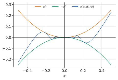
Warm-up example. \(\lim_{x\to0} x^2\sin(1/x)\). We know nothing useful about \(\sin(1/x)\) near 0 — it oscillates wildly — except that it stays between \(-1\) and 1. Multiplying by \(x^2 \ge 0\): Try it: Squeeze x² sin(1/x) to 0.
Both outer functions tend to 0, so \(\lim_{x\to0} x^2\sin(1/x) = 0\). The wild oscillation is crushed by the shrinking factor.
16.6.3. Proof that sin x / x → 1
Take \(0 < x < \frac{\pi}{2}\) and draw an angle \(x\) (in radians) at the centre \(O\) of a unit circle. Let \(A = (1, 0)\), let \(B = (\cos x, \sin x)\) be the point on the circle, and let \(T\) be the point where the line \(OB\) meets the vertical tangent line at \(A\); by similar triangles \(AT = \tan x\). Try it: Tabulate sin x / x.
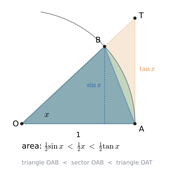
The three regions are nested, so their areas are in order:
(The triangle \(OAB\) has base 1 and height \(\sin x\); the sector has area \(\frac12r^2\theta\) with \(r = 1\), which is where radians are essential; triangle \(OAT\) has base 1 and height \(\tan x\).) Now manipulate:
As \(x \to 0^{+}\), \(\cos x \to 1\). The squeeze theorem gives \(\lim_{x\to0^{+}}\frac{\sin x}{x} = 1\). For negative \(x\), note that \(\frac{\sin(-x)}{-x} = \frac{-\sin x}{-x} = \frac{\sin x}{x}\) (the function is even), so the left-hand limit is the same. Therefore
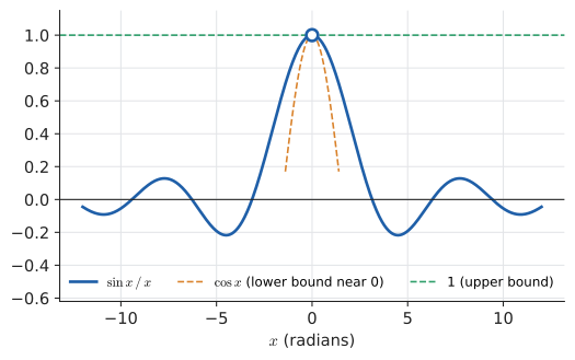
Geometrically: for small angles, the arc length \(x\) and the half-chord \(\sin x\) are almost the same. This is the small-angle approximation \(\sin x \approx x\), used throughout physics and engineering (the simple pendulum, optics, surveying).
16.6.4. Where you’d use this
The small-angle approximation \(\sin x \approx \tan x \approx x\) (radians) turns angles into lengths with no trigonometry.
-
Outdoors and sport: rifle scopes and some binoculars are marked in milliradians (thousandths of a radian). An object of height \(H\) metres that spans \(m\) milliradians is about \(1000H/m\) metres away, since \(H/d \approx \tan(m/1000) \approx m/1000\). A 1.8 m person spanning 3 milliradians is about \(1000 \times 1.8 / 3 = 600\) m away.
-
Astronomy: the Moon spans about 0.52°, which is \(0.52 \times \pi/180 \approx 0.0091\) rad. At a distance of 384,400 km its diameter is about \(384{,}400 \times 0.0091 \approx 3{,}490\) km (the true value is 3,474 km). Telescope and camera specifications ("arcseconds per pixel") are all \(\text{size} \approx \text{distance} \times \text{angle}\).
-
Computing: the function \(\operatorname{sinc} x = \sin x / x\) (with value 1 at 0, using this limit) is the ideal interpolation filter in signal processing. Image-resizing filters such as Lanczos (an option in most image editors and in libraries like Pillow) are built from it, and so is audio sample-rate conversion. The code has to special-case \(x = 0\), and it does that by returning the limit, 1.
16.6.5. Using the result
Worked example. \(\lim_{x\to0}\dfrac{\sin 3x}{x}\). Substitute \(u = 3x\) (so \(u \to 0\) as \(x \to 0\)): Try it: Check this limit.
Worked example. \(\lim_{x\to0}\dfrac{1 - \cos x}{x}\). Multiply by the "conjugate" \(1 + \cos x\): Try it: Check this limit.
These two limits are exactly what is needed in Chapter 17 to show that the derivative of \(\sin x\) is \(\cos x\).
|
Degrees ruin everything
The result \(\frac{\sin x}{x} \to 1\) holds only when \(x\) is in radians. In degrees, \(\sin(x^\circ) = \sin\left(\frac{\pi x}{180}\right)\), so \(\frac{\sin(x^\circ)}{x} \to \frac{\pi}{180} \approx 0.01745\). The area formula \(\frac12r^2\theta\) for a sector also assumes radians. This is the deep reason calculus always uses radians: they are the unit in which \(\sin x \approx x\) for small \(x\). It is also a classic bug: |
16.7. Continuity
16.7.1. The problem
For most functions you meet, the limit at a point is just the value at the point: \(\lim_{x\to2} x^2 = 4 = 2^2\). The interesting cases are where this fails. We want a name for the good behaviour, and a catalogue of the ways it can break.
16.7.2. Intuition
A function is continuous if you can draw its graph without lifting your pen: no holes, no jumps, no vertical asymptotes, no wild oscillations. Small changes in input produce small changes in output. Physical quantities — the temperature in a room over time, the position of a car — are continuous; a step change in price at a tax threshold is not.
|
Continuity at a point
A function \(f\) is continuous at \(a\) if all three conditions hold:
\(f\) is continuous on an interval if it is continuous at every point of it (using one-sided limits at closed endpoints), and simply continuous if it is continuous at every point of its domain. A point where continuity fails is a discontinuity. |
Condition 3 is the heart of it: the limit is what you get by substituting. That is why direct substitution works — it works precisely for continuous functions.
16.7.3. Types of discontinuity
Each condition can fail, giving a catalogue that maps onto the pictures earlier in the chapter:
-
Removable discontinuity (a hole): the limit exists but \(f(a)\) is undefined or different. \(\frac{x^2 - 4}{x - 2}\) at 2. "Removable" because redefining \(f(2) = 4\) repairs it. Similarly, \(\frac{\sin x}{x}\) has a removable discontinuity at 0; the repaired function (defined to be 1 at 0) is called \(\operatorname{sinc} x\) and is important in signal processing.
-
Jump discontinuity: both one-sided limits exist but differ. The floor function at each integer; postage rates; tax brackets.
-
Infinite discontinuity: the function blows up — a vertical asymptote. \(\frac1x\) at 0, \(\tan x\) at \(\frac{\pi}{2}\).
-
Oscillating discontinuity: no one-sided limit exists. \(\sin(1/x)\) at 0.
16.7.4. Which functions are continuous?
A great deal follows from the limit laws:
-
Polynomials are continuous everywhere.
-
Rational functions are continuous everywhere in their domain (i.e. except where the denominator is zero).
-
\(\sqrt[n]{x}\), \(e^x\), \(\ln x\), \(\sin x\), \(\cos x\), \(|x|\) are continuous on their domains.
-
Sums, differences, products, quotients (where the denominator is nonzero), and compositions of continuous functions are continuous.
So \(e^{\sin x} + \sqrt{x^2 + 1}\) is continuous everywhere, with no work. The composition rule also lets limits pass inside continuous functions: \(\lim_{x\to a} g(f(x)) = g\left(\lim_{x\to a} f(x)\right)\) when \(g\) is continuous at the inner limit.
Worked example (making a piecewise function continuous). For which value of \(k\) is
continuous everywhere? Each piece is a polynomial, hence continuous; the only danger is the join at \(x = 2\).
-
\(f(2) = 2k + 1\) (the first piece includes \(x = 2\)).
-
Left limit: \(\lim_{x\to2^-}(kx + 1) = 2k + 1\). Right limit: \(\lim_{x\to2^{+}}(x^2 - 1) = 3\). The limit exists iff \(2k + 1 = 3\).
-
Then it equals \(f(2)\) automatically.
So \(k = 1\).
|
Continuity is about the domain
Is \(\frac1x\) continuous? By the definition, yes: it is continuous at every point of its domain (all \(x \ne 0\)). Its graph has two pieces, but 0 is not in the domain, so there is no point at which continuity fails. Some textbooks nevertheless say "\(\frac1x\) has a discontinuity at 0"; be aware that the phrase is used loosely. What matters for theorems like the IVT below is continuity on a whole interval, and \(\frac1x\) is not continuous on any interval containing 0. |
16.7.5. Where you’d use this
Continuity is the promise that a small change in input gives a small change in output. Discontinuities are where that promise breaks, and they often matter more than the smooth parts.
-
Shopping: an online shop charges $4.99 delivery below $35 and nothing at $35 or more. The total you pay has a jump discontinuity at $35. A $33 basket costs $37.99, but a $35 basket costs $35.00: adding a $2 item gets you more and you pay $2.99 less. Tax bands, parcel weight limits and phone-data caps all create jumps like this, and people (rationally) bunch up just past them.
-
Engineering: in a lift, a robot arm or a roller coaster, a jump in velocity means an impossible infinite acceleration, and in practice a violent jolt. Motion controllers plan paths whose position, velocity and acceleration are all continuous, so that the ride is smooth.
-
Computing: graphics and animation curves (Bézier curves, splines) are joined so that position and direction are continuous where pieces meet. Otherwise you see a kink or a "pop" between frames. In code, a jump discontinuity is usually an
ifstatement, such asif total >= 35:, and the boundary value is exactly where off-by-one and floating-point bugs live: is 34.999999999 less than 35?
16.8. The intermediate value theorem and bisection
16.8.1. The problem
Does \(x^3 - x - 2 = 0\) have a solution? It is a cubic with no rational roots (the candidates \(\pm1, \pm2\) all fail), so factoring will not help. But \(f(1) = 1 - 1 - 2 = -2 < 0\) and \(f(2) = 8 - 2 - 2 = 4 > 0\). The graph of a continuous function cannot get from below the axis to above it without crossing. That intuition is a theorem.
|
Intermediate value theorem
Intermediate value theorem (IVT): if \(f\) is continuous on the closed interval \({[}a, b]\) and \(N\) is any number between \(f(a)\) and \(f(b)\), then there is at least one \(c\) in \({[}a, b]\) with \(f(c) = N\). The most-used special case: if \(f\) is continuous on \({[}a, b]\) and \(f(a)\) and \(f(b)\) have opposite signs, then \(f\) has a root (a zero) somewhere in \((a, b)\). |
The IVT tells you a root exists; it does not tell you where. It also needs continuity: \(f(x) = \frac1x\) has \(f(-1) = -1 < 0 < 1 = f(1)\) but no root, because it is not continuous on \({[}-1, 1]\).
16.8.2. From theorem to algorithm: bisection
The IVT becomes an algorithm with one observation. If there is a sign change on \({[}a, b]\), evaluate \(f\) at the midpoint \(m\). Either \(f(m) = 0\) (done), or the sign change is in \({[}a, m]\), or it is in \({[}m, b]\). Keep the half with the sign change and repeat. The interval known to contain a root halves every step — it is binary search on the real line.
Input: a continuous function \(f\); an interval \({[}a, b]\) with \(f(a)\) and \(f(b)\) of opposite signs; a tolerance \(\varepsilon > 0\).
Steps:
-
Compute the midpoint \(m = \frac{a + b}{2}\) and \(f(m)\).
-
If \(f(m) = 0\) or the half-width \(\frac{b - a}{2} < \varepsilon\), return \(m\).
-
If \(f(a)\) and \(f(m)\) have opposite signs, set \(b \leftarrow m\); otherwise set \(a \leftarrow m\).
-
Go to step 1.
Output: \(m\), within \(\varepsilon\) of a true root. After \(n\) halvings the interval has width \(\frac{b - a}{2^n}\), so about \(\log_2\frac{b - a}{\varepsilon}\) steps are needed.
Worked example by hand. \(f(x) = x^3 - x - 2\) on \({[}1, 2]\). Try it: Step through this table.
| step | \(a\) | \(b\) | midpoint \(m\) | \(f(m)\) | root is in |
|---|---|---|---|---|---|
1 |
1 |
2 |
1.5 |
\(-0.125\) |
\({[}1.5, 2]\) |
2 |
1.5 |
2 |
1.75 |
\(1.609\) |
\({[}1.5, 1.75]\) |
3 |
1.5 |
1.75 |
1.625 |
\(0.666\) |
\({[}1.5, 1.625]\) |
4 |
1.5 |
1.625 |
1.5625 |
\(0.252\) |
\({[}1.5, 1.5625]\) |
5 |
1.5 |
1.5625 |
1.53125 |
\(0.0591\) |
\({[}1.5, 1.53125]\) |
6 |
1.5 |
1.53125 |
1.515625 |
\(-0.0341\) |
\({[}1.515625, 1.53125]\) |
7 |
1.515625 |
1.53125 |
1.5234375 |
\(0.0123\) |
\({[}1.515625, 1.5234375]\) |
(Step 1 in detail: \(f(1.5) = 3.375 - 1.5 - 2 = -0.125\). Since \(f(1.5) < 0 < f(2)\), the root lies in \({[}1.5, 2]\).) After 7 steps the root is pinned inside an interval of width \(2^{-7} \approx 0.0078\): it is about 1.52.
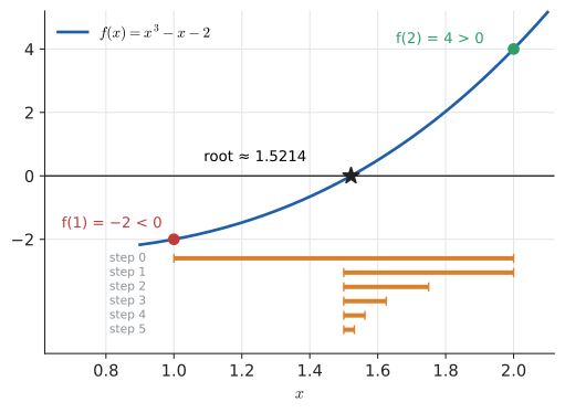
def bisection(f, a, b, tol=1e-10, max_iter=200):
    """Find a root of continuous f in [a, b], given f(a), f(b) of opposite sign."""
    fa, fb = f(a), f(b)
    if fa * fb > 0:
        raise ValueError("f(a) and f(b) must have opposite signs")
    for n in range(max_iter):
        m = (a + b) / 2
        fm = f(m)
        if fm == 0 or (b - a) / 2 < tol:
            return m, n
        if fa * fm < 0:          # sign change in left half
            b, fb = m, fm
        else:                    # sign change in right half
            a, fa = m, fm
    return (a + b) / 2, max_iter

root, steps = bisection(lambda x: x**3 - x - 2, 1, 2)
print(root, steps)
print(root**3 - root - 2)
1.5213797068572603 33 3.131943593359665e-10
33 halvings shrink the interval from width 1 to about \(10^{-10}\), as predicted: \(\log_2 10^{10} \approx 33.2\).
16.8.3. Choosing a root-finding method
-
Bisection is slow (one binary digit per step) but guaranteed: given a continuous function and a sign change, it cannot fail, and you know the error bound in advance.
-
Newton’s method (Chapter 18, Chapter 32) is far faster near a root — the number of correct digits roughly doubles each step — but needs the derivative and can diverge or wander off from a poor starting point.
-
In practice, robust library routines (such as Brent’s method, behind
scipy.optimize.brentq) combine both: fast steps when they behave, bisection as a safety net.
16.8.4. Where you’d use this
-
Finance: you invest $1,000 and get $600 back after one year and another $600 after two. What annual rate of return is that? It’s the rate \(r\) that makes the net present value zero:
\[f(r) = -1000 + \frac{600}{1 + r} + \frac{600}{(1 + r)^2} = 0.\]\(f(0) = 200 > 0\) and \(f(1) = -550 < 0\), and \(f\) is continuous for \(r > -1\), so by the IVT a root lies in between. Bisection finds \(r \approx 0.1307\), a 13.07% annual return. A spreadsheet’s
IRRfunction solves exactly this equation with an iterative root-finder. (Here a quadratic in \(1/(1 + r)\) would also work, but cash flows over 30 years give a degree-30 polynomial, and then iteration is the only practical option.) -
Engineering: "at what speed does this beam start to resonate?", "what pipe diameter gives exactly this flow?" When an equation has no algebraic solution but you can evaluate it and find a sign change, bisection gives a guaranteed answer with a known error bound. Safety-critical code values that guarantee.
-
Computing: "binary search on the answer". What is the largest batch size that fits in GPU memory? Try 512 (fits) and 1,024 (out of memory), then 768, and so on. Nine more tries pin down the exact limit among the 512 sizes in between. That’s bisection on a function that changes from "fits" to "doesn’t fit".
|
When bisection fails
|
|
The IVT in the world
The IVT has surprising everyday consequences. The wobbly table: on any continuous floor (no steps), a square four-legged table can be rotated so all four legs touch the ground — apply the IVT to the height difference of opposite leg pairs as you rotate through \(90^\circ\). Antipodal temperatures: at any moment there are two diametrically opposite points on the equator with exactly the same temperature (apply the IVT to \(T(\theta) - T(\theta + 180^\circ)\), which changes sign over half a turn). And git bisect, which binary-searches the commit history for the first bad commit, relies on a discrete version of the same idea: there is a good commit and a bad commit, so somewhere in between the state must switch. |
|
Bisection stepper
Enter a function and an interval. Each click on "step" shades the current interval, marks the midpoint with the sign of \(f(m)\), and keeps the half containing the sign change. A side panel plots the interval width on a logarithmic scale (a straight line: halving each step). Include a mode with \(1/x\) to watch bisection "converge" to an asymptote. Try it: Bisection on 1/x · Open the bisection stepper |
16.9. Limits at infinity and asymptotes
16.9.1. The problem
What happens to \(f(x)\) as \(x\) grows without bound? This is the question of long-run behaviour: the steady state of a cooling cup of coffee, the terminal velocity of a falling object, the cost of an algorithm on enormous inputs.
|
Limit at infinity
\(\lim_{x\to\infty} f(x) = L\) means \(f(x)\) can be made as close to \(L\) as we like by taking \(x\) sufficiently large. Similarly for \(x \to -\infty\). If such an \(L\) exists, the horizontal line \(y = L\) is a horizontal asymptote. For a sequence (Chapter 14), \(\lim_{n\to\infty} a_n = L\) means the same thing with \(n\) restricted to whole numbers; this is exactly the "convergence" of the previous chapter, now with a name. |
The basic facts: \(\lim_{x\to\infty}\frac{1}{x} = 0\), and more generally \(\lim_{x\to\infty}\frac{1}{x^p} = 0\) for any \(p > 0\). Everything else is reduced to these.
16.9.2. Dividing by the highest power
A rational function at infinity is a \(\frac{\infty}{\infty}\) indeterminate form. The technique: divide numerator and denominator by the highest power of \(x\) in the denominator, so every term becomes a constant or tends to 0.
Worked example. \(\lim_{x\to\infty}\dfrac{3x^2 - 5x + 1}{2x^2 + 7}\). Try it: Limit at infinity, tabulated.
The lesson: at infinity, only the leading terms matter. \(3x^2 - 5x + 1\) "behaves like" \(3x^2\) and \(2x^2 + 7\) like \(2x^2\).
Input: \(\dfrac{p(x)}{q(x)}\) with \(\deg p = m\), \(\deg q = n\), leading coefficients \(a_m\), \(b_n\).
Steps: compare degrees.
-
\(m < n\): the limit is 0 (horizontal asymptote \(y = 0\)).
-
\(m = n\): the limit is \(\dfrac{a_m}{b_n}\), the ratio of leading coefficients.
-
\(m > n\): no finite limit; the function grows like \(\frac{a_m}{b_n}x^{m-n}\), heading to \(\pm\infty\). (If \(m = n + 1\) the graph approaches a slanted line, an oblique asymptote, found by polynomial division.)
To justify any case, divide top and bottom by \(x^n\).
Output: the limit, and the horizontal asymptote if there is one.
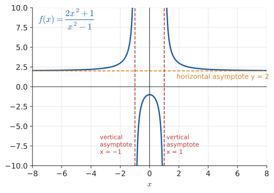
Finding vertical asymptotes. These occur where the denominator is zero but the numerator is not (after cancelling common factors — a common factor gives a hole instead). For
the numerator is never zero, so \(x = 1\) and \(x = -1\) are vertical asymptotes; the degrees are equal, so \(y = \frac{2}{1} = 2\) is the horizontal asymptote.
Worked example (∞ − ∞). \(\lim_{x\to\infty}\left(\sqrt{x^2 + x} - x\right)\). Both terms grow without bound; their difference is indeterminate. Rationalise: Try it: Tabulate √(x²+x) − x.
16.9.3. The growth hierarchy
Beyond polynomials, the essential facts for limits at infinity (proved with tools from Chapter 18) are that, for any constants \(p > 0\) and \(b > 1\),
In words: logarithms grow slower than any power, and powers grow slower than any exponential. \(\ln x\) loses to \(x^{0.01}\) eventually (though "eventually" can be astronomically far out), and \(x^{100}\) loses to \(1.01^x\).
16.9.4. Where you’d use this
Limits at infinity describe where things settle, which is often the only question that matters in the long run.
-
Kitchen physics: a cup of coffee at 90°C in a 20°C room cools according to Newton’s law of cooling, roughly \(T(t) = 20 + 70e^{-0.05t}\) (\(t\) in minutes). After 30 minutes it is \(20 + 70e^{-1.5} \approx 35.6\)°C. As \(t \to \infty\), \(e^{-0.05t} \to 0\), so \(T \to 20\): the room temperature is a horizontal asymptote. Solving \(20 + 70e^{-0.05t} = 25\) gives \(t = 20\ln 14 \approx 52.8\) minutes to get within 5°C of it.
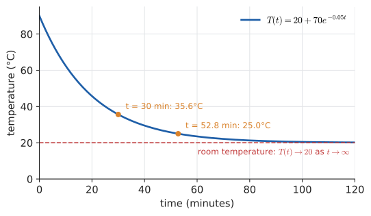 Figure 143. Newton’s law of cooling. The temperature approaches the room’s 20°C (dashed) but never quite reaches it: a horizontal asymptote.
-
Science: a skydiver’s speed approaches a terminal velocity (about 55 m/s, roughly 200 km/h, belly-down) as air resistance grows to match gravity. A charging capacitor’s voltage approaches the supply voltage, and a drug level approaches the steady state from Chapter 14. Each model is "a constant plus a decaying exponential", and the limit is the constant.
-
Business and cloud computing: a service costs $500 a month in fixed fees plus $0.0004 per request. The cost per request is \(\frac{500 + 0.0004n}{n} = \frac{500}{n} + 0.0004\). At a million requests a month that’s $0.0009; at a hundred million it’s $0.000405. As \(n \to \infty\) it tends to $0.0004: fixed costs are spread ever thinner, and only the marginal cost survives. This is "divide by the highest power" again, and it is the arithmetic behind economies of scale.
16.9.5. A famous limit at infinity
Compound interest, compounded ever more frequently, leads to
a \(1^\infty\) indeterminate form: the base tends to 1 but the exponent grows. This is one standard definition of \(e\) (Chapter 12). We will come back to it below, because a computer gets it spectacularly wrong.
16.10. Optional depth: the formal ε–δ definition
|
This section can be skipped on a first reading; nothing later depends on fluency with it. Read it if you want to know what "as close as we like" and "sufficiently close" mean precisely — the step that turned calculus from a brilliant collection of techniques into rigorous mathematics. |
16.10.1. Why "close" needs a definition
For 150 years after Newton and Leibniz, calculus worked spectacularly while its foundations were shaky: quantities were "infinitely small" but not zero, vanishing but not vanished. Bishop Berkeley mocked these as "the ghosts of departed quantities". The resolution, by Cauchy, Bolzano, and above all Weierstrass in the 19th century, was to eliminate the vague words "approaches" and "infinitely small" entirely, replacing them with statements about ordinary inequalities.
16.10.2. The definition as a game
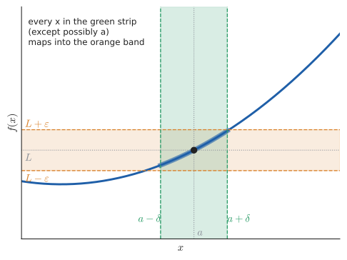
Think of proving \(\lim_{x\to a} f(x) = L\) as a game between a challenger and a prover.
-
The challenger picks a tolerance \(\varepsilon > 0\) (Greek epsilon, for "error"): "I want \(f(x)\) within \(\varepsilon\) of \(L\)."
-
The prover must respond with a distance \(\delta > 0\) (Greek delta, for "distance"): "Then keep \(x\) within \(\delta\) of \(a\) (but not equal to it)."
-
The prover wins the round if every such \(x\) gives \(f(x)\) within \(\varepsilon\) of \(L\).
The limit is \(L\) if the prover can win every round, no matter how small an \(\varepsilon\) the challenger chooses. Usually the prover wins by giving a formula for \(\delta\) in terms of \(\varepsilon\).
|
Limit (formal, ε–δ)
\(\lim_{x\to a} f(x) = L\) means: for every \(\varepsilon > 0\) there exists a \(\delta > 0\) such that
\[0 < |x - a| < \delta \quad\Longrightarrow\quad |f(x) - L| < \varepsilon.\]
Here \(|x - a|\) is the distance between \(x\) and \(a\) (Chapter 5); "\(0 < |x - a|\)" excludes \(x = a\) itself; and \(\Longrightarrow\) reads "implies". In the language of logic (Chapter 21): \(\forall\varepsilon > 0\ \exists\delta > 0\ \forall x\ (0 < |x - a| < \delta \Rightarrow |f(x) - L| < \varepsilon)\). |
16.10.3. Worked examples
A linear function. Prove \(\lim_{x\to3}(2x + 1) = 7\). Try it: Play ε–δ for 2x + 1.
Scratch work (finding \(\delta\)): we need \(|(2x + 1) - 7| < \varepsilon\). Simplify: \(|2x - 6| = 2|x - 3| < \varepsilon\) exactly when \(|x - 3| < \frac{\varepsilon}{2}\). So choose \(\delta = \frac{\varepsilon}{2}\).
Proof: given \(\varepsilon > 0\), let \(\delta = \frac{\varepsilon}{2}\). If \(0 < |x - 3| < \delta\), then
The slope 2 means outputs move twice as fast as inputs, so the input window must be half as wide as the output window. If the challenger demands \(\varepsilon = 0.001\), the prover answers \(\delta = 0.0005\).
A quadratic. Prove \(\lim_{x\to2}x^2 = 4\). Try it: Play ε–δ for x².
Scratch work: \(|x^2 - 4| = |x - 2|\,|x + 2|\). The factor \(|x - 2|\) is what we control; the factor \(|x + 2|\) varies, so we bound it. If we insist \(\delta \le 1\), then \(|x - 2| < 1\) means \(1 < x < 3\), so \(|x + 2| < 5\). Then \(|x^2 - 4| < 5|x - 2|\), which is below \(\varepsilon\) when \(|x - 2| < \frac{\varepsilon}{5}\).
Proof: given \(\varepsilon > 0\), let \(\delta = \min\left(1, \frac{\varepsilon}{5}\right)\). If \(0 < |x - 2| < \delta\), then \(|x + 2| < 5\) (because \(\delta \le 1\)) and
Sequences: the ε–N version. For sequences the "closeness of input" is replaced by "far enough along": \(\lim_{n\to\infty} a_n = L\) means for every \(\varepsilon > 0\) there is an \(N\) such that \(|a_n - L| < \varepsilon\) for all \(n > N\). Example: \(\frac1n \to 0\), because given \(\varepsilon\), any \(N \ge \frac{1}{\varepsilon}\) works: \(n > N\) gives \(\frac1n < \frac1N \le \varepsilon\).
|
The ε–δ game
The app plays challenger: it shows a graph, a point \(a\), a claimed limit \(L\), and a horizontal band of half-height \(\varepsilon\). The user drags a vertical strip of half-width \(\delta\); the portion of the graph inside the strip turns green if it fits within the band and red where it escapes. Each round, \(\varepsilon\) shrinks. For a function with a jump, the user discovers that no \(\delta\) works once \(\varepsilon\) is smaller than half the jump — a visual proof that the limit does not exist. Try it: Try to win at a jump · Play the ε–δ game |
16.11. Limits meet the computer
Limits are about what happens as something gets arbitrarily small or large. Computers have neither arbitrarily small nor arbitrarily large numbers. This gap is where many numerical bugs live.
16.11.1. Why you cannot just plug in h = 1e-20
The car example suggests a tempting shortcut for computing a derivative: just evaluate the average rate of change with a tiny \(h\). Try it on \(\sin\) at \(x = 1\), where the true answer is \(\cos 1 \approx 0.5403023\): Try it: Shrink h yourself.
import math

x = 1.0
exact = math.cos(x)              # the true rate of change of sin at x = 1
for k in [1, 2, 4, 6, 8, 10, 12, 14, 16, 20]:
    h = 10.0 ** (-k)
    approx = (math.sin(x + h) - math.sin(x)) / h
    print(f"h = 1e-{k:<2}  approx = {approx:.15f}  error = {abs(approx - exact):.1e}")
print(1.0 + 1e-20 == 1.0)
h = 1e-1 approx = 0.497363752535389 error = 4.3e-02 h = 1e-2 approx = 0.536085981011869 error = 4.2e-03 h = 1e-4 approx = 0.540260231418621 error = 4.2e-05 h = 1e-6 approx = 0.540301885121330 error = 4.2e-07 h = 1e-8 approx = 0.540302291796024 error = 1.4e-08 h = 1e-10 approx = 0.540302247387103 error = 5.8e-08 h = 1e-12 approx = 0.540345546085064 error = 4.3e-05 h = 1e-14 approx = 0.544009282066327 error = 3.7e-03 h = 1e-16 approx = 0.000000000000000 error = 5.4e-01 h = 1e-20 approx = 0.000000000000000 error = 5.4e-01 True
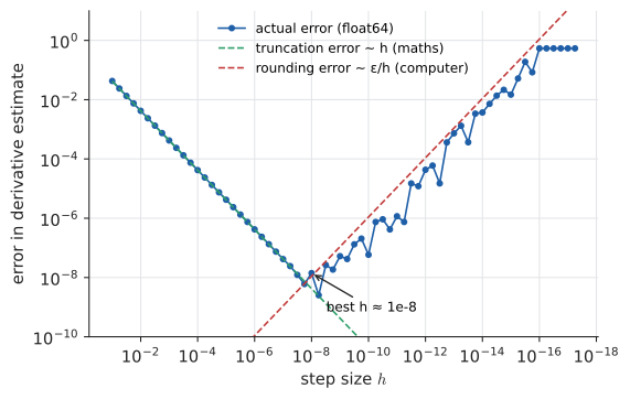
Mathematically, shrinking \(h\) always helps. Computationally, the error falls until \(h \approx 10^{-8}\) and then rises, until at \(h = 10^{-16}\) the answer is 0 — completely wrong. Two errors compete:
-
Truncation error (the mathematics): the secant slope differs from the tangent slope by an amount roughly proportional to \(h\). Shrinking \(h\) reduces it.
-
Rounding error (the computer): a double carries about 16 significant digits (machine epsilon \(\approx 2.2\times10^{-16}\)). \(\sin(1 + h)\) and \(\sin 1\) agree in their first many digits, so subtracting them cancels those digits and leaves mostly noise (catastrophic cancellation); dividing by a tiny \(h\) then magnifies that noise, roughly like \(\frac{10^{-16}}{h}\).
At \(h = 10^{-20}\) it is worse still: \(1 + 10^{-20}\) rounds to exactly \(1.0\) (the last line prints True), so the numerator is exactly zero. The best compromise is around \(h \approx \sqrt{\text{machine epsilon}} \approx 10^{-8}\), giving only about 8 correct digits. Better formulas (central differences), and better approaches altogether (automatic differentiation, as used in every ML framework), are the subject of Chapter 32.
The \((1 + \frac1n)^n \to e\) limit fails in the same way: Try it: Watch (1 + 1/n)ⁿ collapse.
import math
for k in [1, 3, 6, 9, 12, 15, 16, 17]:
    n = 10**k
    print(f"n = 1e{k:<2}  (1 + 1/n)^n = {(1 + 1/n)**n:.12f}")
print("e          =", f"{math.e:.12f}")
n = 1e1 (1 + 1/n)^n = 2.593742460100 n = 1e3 (1 + 1/n)^n = 2.716923932236 n = 1e6 (1 + 1/n)^n = 2.718280469096 n = 1e9 (1 + 1/n)^n = 2.718282052012 n = 1e12 (1 + 1/n)^n = 2.718523496037 n = 1e15 (1 + 1/n)^n = 3.035035206549 n = 1e16 (1 + 1/n)^n = 1.000000000000 n = 1e17 (1 + 1/n)^n = 1.000000000000 e = 2.718281828459
Approaching \(e\) nicely, then drifting away, then collapsing to 1 once \(1 + 10^{-16}\) rounds to 1. The mathematical limit is a statement about exact arithmetic. Floating point approximates it well only in a middle range. This is why library functions like math.log1p and math.expm1 exist: they compute \(\ln(1 + x)\) and \(e^x - 1\) accurately for tiny \(x\) without forming \(1 + x\).
|
Precision runs out before the limit does
Whenever code takes a limit by brute force — a tiny \(h\), a huge \(n\), iterating "until it converges" — check for cancellation (subtracting nearly equal numbers) and absorption (adding a tiny number to a large one). Plotting the error against the parameter on log–log axes, as above, is the quickest diagnosis: a V shape means rounding error has taken over. |
16.11.2. Convergence of iterative algorithms
Many algorithms produce a sequence of approximations \(x_0, x_1, x_2, \ldots\) that should converge to the answer: square roots, Newton’s method, gradient descent, PageRank, iterative linear solvers. "The algorithm converges" means precisely \(\lim_{n\to\infty}x_n = x^*\). Heron’s ancient method for \(\sqrt a\) iterates \(x_{n+1} = \frac12\left(x_n + \frac{a}{x_n}\right)\) (if \(x_n\) is too big, \(\frac{a}{x_n}\) is too small, so average them):
def heron_sqrt(a, x0=1.0, tol=1e-15, max_iter=60):
    x = x0
    for n in range(1, max_iter + 1):
        x_new = (x + a / x) / 2
        print(n, f"{x_new:.16f}", f"{abs(x_new - x):.1e}")
        if abs(x_new - x) <= tol * abs(x_new):
            return x_new
        x = x_new
    raise RuntimeError("did not converge")

heron_sqrt(2)
Try it: Step Heron’s method for √2.
1 1.5000000000000000 5.0e-01
2 1.4166666666666665 8.3e-02
3 1.4142156862745097 2.5e-03
4 1.4142135623746899 2.1e-06
5 1.4142135623730949 1.6e-12
6 1.4142135623730949 0.0e+00
Three practical lessons follow from the limit concept:
-
Stopping criteria. We never reach the limit; we stop when successive iterates differ by less than a tolerance, ideally a relative one (
tol * abs(x_new)), since an absolute tolerance of \(10^{-15}\) is meaningless for numbers near \(10^{20}\). -
Guard against non-convergence. A
max_itercap turns "this sequence has no limit" from an infinite loop into an error. -
Rate of convergence. The step sizes above go \(5\times10^{-1}, 8\times10^{-2}, 2.5\times10^{-3}, 2\times10^{-6}, 1.6\times10^{-12}\): the number of correct digits doubles each step (quadratic convergence). Bisection, by contrast, gains a constant factor of 2 per step (linear convergence). These rates are themselves defined by limits, such as \(\lim \frac{|e_{n+1}|}{|e_n|^2}\), and are studied in Chapter 32.
16.11.3. Asymptotic analysis is limits at infinity
Big-O notation, used informally in Chapter 14, is really a statement about limits at infinity. To compare a cost function \(f(n)\) with a reference function \(g(n)\), look at the ratio:
(The precise definition, \(f = O(g)\) if \(f(n) \le C g(n)\) for some constant \(C\) and all large \(n\), does not require the limit to exist, but when it does exist, this test settles the question.)
import math

costs = {
    "3n^2 + 10n": lambda n: 3 * n**2 + 10 * n,
    "n log2 n": lambda n: n * math.log2(n),
    "n^1.5": lambda n: n ** 1.5,
}
g = lambda n: n**2
for n in [10, 1000, 10**6]:
    row = [f"{name}: {f(n) / g(n):.6f}" for name, f in costs.items()]
    print(f"n = {n:>7}  ratio to n^2 ->  " + "   ".join(row))
n = 10 ratio to n^2 -> 3n^2 + 10n: 4.000000 n log2 n: 0.332193 n^1.5: 0.316228 n = 1000 ratio to n^2 -> 3n^2 + 10n: 3.010000 n log2 n: 0.009966 n^1.5: 0.031623 n = 1000000 ratio to n^2 -> 3n^2 + 10n: 3.000010 n log2 n: 0.000020 n^1.5: 0.001000
\(\frac{3n^2 + 10n}{n^2} = 3 + \frac{10}{n} \to 3\), so \(3n^2 + 10n = \Theta(n^2)\): the "divide by the highest power" technique, applied to algorithm costs. \(\frac{n\log n}{n^2} = \frac{\log n}{n} \to 0\), so \(n\log n = o(n^2)\): the growth hierarchy (logs lose to powers) is why \(O(n\log n)\) sorting beats \(O(n^2)\) sorting for large inputs, whatever the constant factors.
|
Floating-point limits
A slider for \(h\) from \(10^{-1}\) to \(10^{-20}\) (log scale) computes the difference quotient of a chosen function in double precision and in exact rational arithmetic side by side, plotting both errors on log–log axes. Show the bits of \(x + h\) and \(x\) as \(h\) shrinks, highlighting the moment they become identical. |
|
Who invented the limit?
Archimedes (c. 250 BCE) computed the area of a parabolic segment and bounds for \(\pi\) by squeezing the unknown between ever-closer inner and outer polygons — the squeeze theorem in all but name. Newton spoke of "prime and ultimate ratios" of "evanescent quantities"; Leibniz of infinitesimals. Cauchy (1821) put the limit at the centre of calculus, and Weierstrass (1850s–60s) gave the ε–δ form used today. Infinitesimals made a comeback in 1961, when Abraham Robinson’s non-standard analysis made them rigorous — so Leibniz’s intuition was vindicated after 300 years. |
16.12. Interactive tools
Browser tools on the companion website that go with this chapter. Each example link in the chapter opens one of them with that example already set up.
16.13. Exercises
Recognition
-
Use the graph of \(f(x) = \frac{|x|}{x}\) to state \(\lim_{x\to0^-}f(x)\), \(\lim_{x\to0^{+}}f(x)\), and whether \(\lim_{x\to0}f(x)\) exists.
-
For each, state which condition of continuity fails at the given point and name the type of discontinuity: (a) \(\frac{x^2 - 1}{x - 1}\) at 1 (b) \(\lfloor x\rfloor\) at 3 (c) \(\frac{1}{(x - 2)^2}\) at 2.
-
Which of these limits are indeterminate forms on substitution? (a) \(\lim_{x\to1}\frac{x^2 - 1}{x - 1}\) (b) \(\lim_{x\to1}\frac{x^2 + 1}{x - 1}\) (c) \(\lim_{x\to0}\frac{\tan x}{x}\).
Application
-
Evaluate: (a) \(\lim_{x\to-2}\frac{x^2 + 5x + 6}{x + 2}\) (b) \(\lim_{x\to4}\frac{\sqrt x - 2}{x - 4}\) (c) \(\lim_{h\to0}\frac{(3 + h)^2 - 9}{h}\).
-
Evaluate: (a) \(\lim_{x\to0}\frac{\sin5x}{\sin2x}\) (b) \(\lim_{x\to0}\frac{\tan x}{x}\) (c) \(\lim_{x\to0}\frac{1 - \cos x}{x^2}\).
-
Evaluate: (a) \(\lim_{x\to\infty}\frac{4x^3 - x}{2x^3 + 5x^2}\) (b) \(\lim_{x\to\infty}\frac{7x + 2}{x^2 + 1}\) (c) \(\lim_{x\to-\infty}\frac{x^2}{3x + 1}\).
-
Find all vertical and horizontal asymptotes of \(f(x) = \frac{x^2 - 4}{x^2 - 3x + 2}\).
-
Find \(c\) so that \(f(x) = x^2\) for \(x < 1\), \(f(x) = 3x - c\) for \(x \ge 1\) is continuous.
Problem solving
-
Show that \(\cos x = x\) has a solution in \({[}0, \frac{\pi}{2}]\), then perform three steps of bisection by hand. Try it: Check your three bisection steps.
-
How many bisection steps are needed to locate a root in \({[}0, 4]\) to within \(10^{-6}\)?
-
Use the squeeze theorem to find \(\lim_{x\to\infty}\frac{\sin x}{x}\).
-
(ε–δ) Prove that \(\lim_{x\to-1}(5 - 3x) = 8\). What \(\delta\) works for \(\varepsilon = 0.03\)?
-
A program computes \(f'(x)\) using \(\frac{f(x + h) - f(x)}{h}\) with \(h = 10^{-15}\) and gets nonsense. Explain why, and suggest a better \(h\).
Answers
-
Left limit \(-1\), right limit \(1\); they differ, so the two-sided limit does not exist.
-
(a) \(f(1)\) is undefined (condition 1); the limit is 2 — removable. (b) \(\lfloor 3\rfloor = 3\) is defined, but the left limit is 2 and the right limit is 3, so the limit does not exist (condition 2) — jump. (c) \(f(2)\) undefined and the function blows up to \(+\infty\) — infinite discontinuity.
-
(a) \(\frac00\): indeterminate. (b) \(\frac{2}{0}\): not indeterminate — the limit does not exist (\(-\infty\) from the left, \(+\infty\) from the right). (c) \(\frac00\): indeterminate.
-
(a) \(\frac{(x + 2)(x + 3)}{x + 2} = x + 3 \to 1\). (b) Multiply by \(\sqrt x + 2\): \(\frac{x - 4}{(x - 4)(\sqrt x + 2)} = \frac{1}{\sqrt x + 2} \to \frac14\). (c) \(\frac{9 + 6h + h^2 - 9}{h} = 6 + h \to 6\) — this is the slope of \(x^2\) at \(x = 3\), a derivative.
-
(a) \(\frac{\sin5x}{\sin2x} = \frac{\sin 5x}{5x}\cdot\frac{2x}{\sin2x}\cdot\frac{5}{2} \to 1\cdot1\cdot\frac52 = \frac52\). (b) \(\frac{\tan x}{x} = \frac{\sin x}{x}\cdot\frac{1}{\cos x} \to 1\cdot1 = 1\). (c) \(\frac{1 - \cos x}{x^2} = \frac{\sin^2 x}{x^2(1 + \cos x)} = \left(\frac{\sin x}{x}\right)^2\frac{1}{1 + \cos x} \to 1\cdot\frac12 = \frac12\).
-
(a) Equal degrees: \(\frac{4}{2} = 2\). (b) Numerator degree lower: 0. (c) Numerator degree higher: \(\frac{x^2}{3x + 1} = \frac{x}{3 + 1/x}\); as \(x \to -\infty\) this tends to \(-\infty\) (no finite limit).
-
\(\frac{(x - 2)(x + 2)}{(x - 1)(x - 2)}\). The factor \(x - 2\) cancels, so \(x = 2\) is a hole (where the limit is \(\frac{4}{1} = 4\)), not an asymptote. Vertical asymptote: \(x = 1\). Equal degrees, leading coefficients 1 and 1: horizontal asymptote \(y = 1\).
-
Left limit at 1: \(1^2 = 1\). Right limit and value: \(3 - c\). Need \(3 - c = 1\), so \(c = 2\).
-
Let \(g(x) = \cos x - x\), continuous. \(g(0) = 1 > 0\), \(g(\frac{\pi}{2}) = -\frac{\pi}{2} < 0\); by the IVT there is a root. Bisection on \({[}0, 1.5708]\): \(m = 0.7854\), \(g(m) = 0.7071 - 0.7854 = -0.0783 < 0\) → \({[}0, 0.7854]\). \(m = 0.3927\), \(g = 0.9239 - 0.3927 = 0.5312 > 0\) → \({[}0.3927, 0.7854]\). \(m = 0.5890\), \(g = 0.8315 - 0.5890 = 0.2425 > 0\) → \({[}0.5890, 0.7854]\). (The root is about 0.7391.)
-
Need \(\frac{4}{2^n} \le 10^{-6}\), i.e. \(2^n \ge 4\times10^6\), \(n \ge \log_2(4\times10^6) \approx 21.9\). So 22 steps (one or two fewer if you return the midpoint and count half-widths).
-
For \(x > 0\): \(-\frac1x \le \frac{\sin x}{x} \le \frac1x\), and both bounds tend to 0. So the limit is 0. (Contrast \(x \to 0\), where the limit is 1.)
-
\(|(5 - 3x) - 8| = |-3x - 3| = 3|x + 1|\). Given \(\varepsilon\), take \(\delta = \frac{\varepsilon}{3}\): then \(0 < |x + 1| < \delta\) gives \(|(5 - 3x) - 8| < 3\delta = \varepsilon\). For \(\varepsilon = 0.03\), \(\delta = 0.01\) (or anything smaller).
-
\(f(x + h)\) and \(f(x)\) agree in nearly all of their roughly 16 significant digits, so their difference is dominated by rounding error of size about \(10^{-16}|f(x)|\); dividing by \(h = 10^{-15}\) makes that error of order 0.1 — as large as the answer. Use \(h \approx 10^{-8}\) (times the scale of \(x\)), or a central difference \(\frac{f(x + h) - f(x - h)}{2h}\) with \(h \approx 10^{-5}\), or automatic differentiation.
16.14. Mastery check
-
Explain in two or three sentences why the instantaneous speed of a car is defined as a limit, and why we cannot simply substitute \(h = 0\) into the average-speed formula.
-
Evaluate \(\lim_{x\to5}\dfrac{x^2 - 25}{x^2 - 4x - 5}\).
-
Evaluate \(\lim_{x\to0}\dfrac{\sqrt{1 + x} - 1}{x}\).
-
Evaluate \(\lim_{x\to0}\dfrac{\sin 4x}{3x}\) and \(\lim_{x\to\infty}\dfrac{5x^2 - 3}{2 - x^2}\).
-
State the three conditions for continuity at \(a\), and decide whether \(f(x) = \frac{x^2 - x}{x}\) (for \(x \ne 0\)), \(f(0) = -1\) is continuous at 0.
-
Use the IVT to show \(x^5 + x - 1 = 0\) has a root in \({[}0, 1]\), and give the first two bisection intervals.
-
Find \(\lim_{n\to\infty}\dfrac{2n^2 + n\log_2 n}{n^2}\), and say what it tells you about the running time \(2n^2 + n\log_2 n\).
Decision rule: All correct without hesitation → move on to Chapter 17. Stuck on 1 → reread Section 16.1 and Section 16.2. Stuck on 2–4 → reread Section 16.5, Section 16.6, and Section 16.9. Stuck on 5–6 → reread Section 16.7 and Section 16.8. Then work the section exercises.
Mastery check answers
-
Instantaneous speed is not a ratio of two measurable changes (over an instant both are zero), so we define it as the value the average speed \(\frac{d(t + h) - d(t)}{h}\) approaches as the interval \(h\) shrinks. Substituting \(h = 0\) gives \(\frac00\), which is meaningless; the limit asks what happens near \(h = 0\), never at it.
-
\(\frac{(x - 5)(x + 5)}{(x - 5)(x + 1)} = \frac{x + 5}{x + 1} \to \frac{10}{6} = \frac53\).
-
Multiply by the conjugate: \(\frac{(1 + x) - 1}{x(\sqrt{1 + x} + 1)} = \frac{1}{\sqrt{1 + x} + 1} \to \frac12\).
-
\(\frac{\sin4x}{3x} = \frac43\cdot\frac{\sin4x}{4x} \to \frac43\). Dividing by \(x^2\): \(\frac{5 - 3/x^2}{2/x^2 - 1} \to \frac{5}{-1} = -5\).
-
(1) \(f(a)\) defined; (2) \(\lim_{x\to a}f(x)\) exists; (3) they are equal. Here \(f(0) = -1\) is defined, and for \(x \ne 0\), \(f(x) = x - 1 \to -1\). The limit equals \(f(0)\), so \(f\) is continuous at 0. (The definition of \(f(0)\) repairs what would otherwise be a removable discontinuity.)
-
\(g(x) = x^5 + x - 1\) is a polynomial, hence continuous; \(g(0) = -1 < 0\), \(g(1) = 1 > 0\), so a root exists in \((0, 1)\). \(g(0.5) = 0.03125 + 0.5 - 1 = -0.469 < 0\) → \({[}0.5, 1]\); \(g(0.75) = 0.2373 + 0.75 - 1 = -0.0127 < 0\) → \({[}0.75, 1]\). (The root is about 0.7549.)
-
\(2 + \frac{\log_2 n}{n} \to 2 + 0 = 2\). A finite, nonzero limit: the running time is \(\Theta(n^2)\); the \(n\log n\) term is negligible for large \(n\).