Volume 1: Foundations to Precalculus · Part IV: Functions, Trigonometry, and Precalculus
Chapter 15. Complex Numbers
Chapter map: the equation \(x^2 + 1 = 0\) has no real solution. Inventing a number \(i\) with \(i^2 = -1\) looks like a cheat, yet it produces a number system in which every polynomial equation can be solved, multiplication becomes rotation, and trigonometry, exponentials, and geometry turn out to be one subject. This chapter builds complex numbers from the arithmetic up to Euler’s formula, De Moivre’s theorem, and roots of unity, then shows them at work in circuits, signals, graphics, the FFT, and the Mandelbrot set.
Why this chapter matters: you will never pay for groceries with \(3 + 2i\), but you use complex numbers every day without seeing them. Your phone’s 4G and Wi-Fi signals encode data as points in the complex plane, the mains electricity in your house is designed with phasors, every MP3 and JPEG went through a Fourier transform built from roots of unity, and every game engine that rotates a sprite is multiplying by \(e^{i\theta}\) under another name. Complex numbers are the natural language for anything that rotates or oscillates, and they turn pages of trigonometry into one line of algebra.
15.1. The problem: equations with no solutions
15.1.1. Two stories
The modern version. Solve \(x^2 + 1 = 0\). Rearranging gives \(x^2 = -1\). But the square of any real number is non-negative: \(3^2 = 9\), \((-3)^2 = 9\), \(0^2 = 0\). No real number squares to \(-1\). The parabola \(y = x^2 + 1\) floats entirely above the x-axis, never touching it. In Chapter 8 this is the case of a negative discriminant, and we said "no real roots". The word real was doing a lot of work there.
The historical version. Complex numbers were not invented to solve \(x^2 + 1 = 0\). Mathematicians were perfectly happy to say that equation had no solution, just as \(x + 5 = 2\) once "had no solution" before negative numbers were accepted. What forced the issue was the cubic. In 1545 Gerolamo Cardano published a formula for solving cubics. Applied to
the formula produces
Square roots of negative numbers! Yet this equation obviously has a real solution: \(x = 4\) works, because \(4^3 = 64 = 15 \cdot 4 + 4\). Around 1572 Rafael Bombelli had what he called "a wild thought". He treated \(\sqrt{-1}\) as a symbol obeying ordinary algebra plus the rule \((\sqrt{-1})^2 = -1\), and noticed that
So \(\sqrt[3]{2 + \sqrt{-121}} = 2 + \sqrt{-1}\), and similarly \(\sqrt[3]{2 - \sqrt{-121}} = 2 - \sqrt{-1}\). Adding, the imaginary parts cancel and \(x = 4\). The "impossible" numbers were a necessary bridge between a real question and a real answer. That is the lesson of this chapter in miniature: complex numbers are a tool for getting real answers.
15.1.2. Intuition: extending the number line again
You have done this before. Natural numbers cannot solve \(x + 5 = 2\), so we invented negatives. Integers cannot solve \(3x = 2\), so we invented fractions. Rationals cannot solve \(x^2 = 2\), so we filled in the irrationals (Chapter 1). Each time, the new numbers were initially distrusted ("negative", "irrational", and now "imaginary" are all slightly insulting names) and each time the extension kept all the old rules working.
The difference this time is geometric. The real numbers fill a line. There is no room left on the line for a number whose square is negative. So the new numbers must live off the line — in a plane.
15.2. The imaginary unit and complex arithmetic
15.2.1. Definitions
|
Imaginary unit
The imaginary unit \(i\) is a number with the defining property \(i^2 = -1\). (Electrical engineers write \(j\), since \(i\) means current; so does Python.) The square roots of a negative number \(-a\) (with \(a > 0\)) are \(\pm i\sqrt{a}\); for example \(\sqrt{-9} = 3i\). |
|
Complex number, real part, imaginary part
A complex number is an expression \(z = a + bi\) where \(a\) and \(b\) are real numbers. \(a\) is the real part, written \(\operatorname{Re}(z)\); \(b\) is the imaginary part, written \(\operatorname{Im}(z)\). Note that the imaginary part is the real number \(b\), not \(bi\). The set of all complex numbers is written \(\mathbb{C}\). Two complex numbers are equal exactly when their real parts are equal and their imaginary parts are equal. A number with \(b = 0\) is real; a number with \(a = 0\), \(b \ne 0\) is called purely imaginary. |
The form \(a + bi\) is called rectangular (or Cartesian, or algebraic) form. "Complex" here means "composite" — made of two parts — not "complicated".
15.2.2. Arithmetic: ordinary algebra plus one rule
The whole of complex arithmetic is: treat \(i\) as an unknown, do ordinary algebra, and replace \(i^2\) by \(-1\) whenever it appears.
Addition and subtraction combine real parts and imaginary parts separately, like collecting like terms:
Multiplication expands the brackets (the distributive law, Chapter 4):
Do not memorise that last line; just expand and simplify each time.
Worked example. Compute \((2 + 3i)(4 - i)\). Try it: Multiply (2 + 3i)(4 − i) visually.
15.2.3. Powers of i
Since \(i^2 = -1\), the powers of \(i\) cycle with period 4:
To compute \(i^n\), divide \(n\) by 4 and keep the remainder (Chapter 23): \(i^{2026} = i^{4\cdot506 + 2} = i^2 = -1\). Negative powers too: \(i^{-1} = \frac{1}{i} = \frac{i}{i^2} = -i\) (multiply top and bottom by \(i\)).
The cycle of four is a strong hint about geometry: something that returns to where it started after four steps sounds like a quarter-turn. We will confirm that shortly.
|
Square roots of negatives do not obey the usual rule
For positive reals \(\sqrt{a}\sqrt{b} = \sqrt{ab}\). Apply it to negatives and you get nonsense:
\[-1 = i \cdot i = \sqrt{-1}\cdot\sqrt{-1} \overset{?}{=} \sqrt{(-1)(-1)} = \sqrt{1} = 1.\]
The faulty step is the "?". The rule \(\sqrt{a}\sqrt{b} = \sqrt{ab}\) is only guaranteed for non-negative \(a, b\). The safe habit: convert \(\sqrt{-a}\) to \(i\sqrt{a}\) first, then compute. So \(\sqrt{-4}\cdot\sqrt{-9} = 2i\cdot3i = 6i^2 = -6\). |
15.3. The complex plane
15.3.1. Intuition: a number is a point
A complex number \(a + bi\) is determined by two real numbers, so it can be pictured as the point \((a, b)\) in a plane. The horizontal axis holds the real numbers (the real axis); the vertical axis holds the purely imaginary numbers (the imaginary axis). This picture is the complex plane, or Argand diagram (after Jean-Robert Argand, 1806, although Caspar Wessel published it first in 1799).
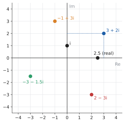
The real number line is still there, intact, as the horizontal axis. Complex numbers did not replace the reals; they surround them.
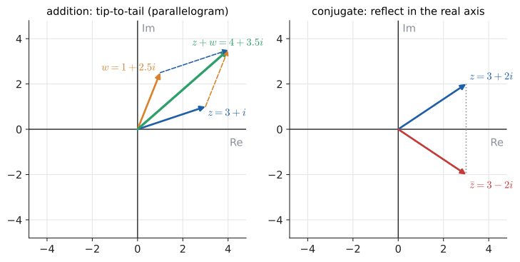
Addition now has a familiar picture: adding complex numbers is adding vectors (Chapter 26), tip to tail. Subtraction \(z - w\) is the arrow from \(w\) to \(z\), so \(|z - w|\) (defined next) is the distance between them. Try it: Add complex numbers as vectors.
15.3.2. Modulus and argument
A point in the plane can be described by its coordinates \((a, b)\) or by its distance from the origin and direction (Chapter 13). For complex numbers these get special names.
|
Modulus and argument
The modulus (or absolute value, or magnitude) of \(z = a + bi\) is its distance from 0: \(|z| = \sqrt{a^2 + b^2}\) (Pythagoras). For a real number it agrees with the ordinary absolute value. The argument \(\arg z\) is the angle from the positive real axis to the arrow for \(z\), measured anticlockwise, usually in radians. It is defined only for \(z \ne 0\) and only up to adding multiples of \(2\pi\). The principal argument is the choice in \((-\pi, \pi]\). |
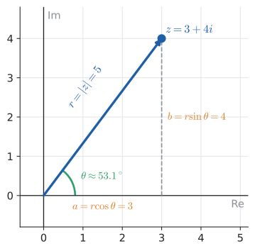
For \(z = 3 + 4i\): \(|z| = \sqrt{9 + 16} = 5\), and \(\tan\theta = \frac43\), so \(\theta = \arctan\frac43 \approx 0.9273\) rad \(\approx 53.13^\circ\).
15.3.3. The method: finding the argument safely
Input: a nonzero complex number \(z = a + bi\).
Steps:
-
Modulus: \(r = \sqrt{a^2 + b^2}\).
-
Plot the point roughly, to see which quadrant it lies in.
-
Compute the reference angle \(\alpha = \arctan\left|\frac{b}{a}\right|\) (if \(a = 0\), the point is on the imaginary axis: \(\theta = \pm\frac{\pi}{2}\)).
-
Adjust for the quadrant: first quadrant \(\theta = \alpha\); second \(\theta = \pi - \alpha\); third \(\theta = -(\pi - \alpha)\); fourth \(\theta = -\alpha\).
-
Check: \(r\cos\theta\) should equal \(a\) and \(r\sin\theta\) should equal \(b\).
Output: \(r = |z|\) and \(\theta = \arg z \in (-\pi, \pi]\).
In code, steps 3–4 are exactly math.atan2(b, a), which is what cmath.phase uses.
Worked example. Find the modulus and argument of \(z = -1 - i\). Try it: Find arg(−1 − i) safely.
-
\(r = \sqrt{(-1)^2 + (-1)^2} = \sqrt2\).
-
The point \((-1, -1)\) is in the third quadrant.
-
Reference angle \(\alpha = \arctan 1 = \frac{\pi}{4}\).
-
Third quadrant: \(\theta = -(\pi - \frac{\pi}{4}) = -\frac{3\pi}{4}\) (that is, \(-135^\circ\)).
-
Check: \(\sqrt2\cos(-\frac{3\pi}{4}) = \sqrt2\cdot(-\frac{\sqrt2}{2}) = -1\) ✓, and the same for the sine ✓.
|
arctan(b/a) is in the wrong quadrant half the time
For \(-1 - i\), a calculator’s \(\arctan\frac{b}{a} = \arctan\frac{-1}{-1} = \arctan 1 = \frac{\pi}{4}\) — pointing into the first quadrant, exactly opposite the true direction. The ratio \(b/a\) has thrown away the signs of \(a\) and \(b\) separately. Always sketch the point, or use the two-argument |
Try it: See arctan(b/a) point wrong.
15.3.4. Where you’d use this
The complex plane earns its keep because \(|z - w|\) is the distance between two points and adding is moving.
-
Your phone’s signal: 4G, 5G and Wi-Fi transmit each group of bits as one complex number, a point in the plane called a symbol. In 16-QAM the 16 allowed points are \(a + bi\) with \(a, b \in \{-3, -1, 1, 3\}\), so each symbol carries 4 bits. Noise shifts the received point slightly. If \(2.8 - 1.2i\) arrives, the receiver decodes it as the nearest allowed point, here \(3 - i\), at distance \(|(2.8 - 1.2i) - (3 - i)| = |-0.2 - 0.2i| \approx 0.28\). The next-nearest points, \(1 - i\) and \(3 - 3i\), are about 1.8 away. Faster Wi-Fi standards pack in more points (1024-QAM carries 10 bits per symbol), which only works when there is less noise. Try it: Decode a 16-QAM symbol.
-
Computing: storing 2D positions as complex numbers turns geometry into arithmetic, and Python’s built-in
complextype is a free 2D vector. Moving is adding, distance isabs(z - w), and direction iscmath.phase(z - w). Programmers solving grid puzzles often store a position aszand a heading asd. Then "step forward" isz += d, "turn left" isd *= 1jand "turn right" isd *= -1j, with noifstatements at all.
15.4. Conjugates and division
15.4.1. The problem
Addition, subtraction, and multiplication are straightforward. What is \(\frac{3 + 4i}{1 - 2i}\)? We need to put it in the form \(a + bi\), which means getting rid of \(i\) in the denominator. This is the same problem as rationalising a denominator like \(\frac{1}{1 + \sqrt2}\), and the same trick solves it.
|
Complex conjugate
The complex conjugate of \(z = a + bi\) is \(\bar z = a - bi\) (also written \(z^*\), especially in physics). Geometrically it is the reflection of \(z\) in the real axis. Key facts:
|
15.4.2. The method
Input: \(\dfrac{z}{w}\) with \(w = c + di \ne 0\).
Steps:
-
Multiply numerator and denominator by \(\bar w = c - di\) (this is multiplying by 1, so the value is unchanged).
-
The denominator becomes \(w\bar w = c^2 + d^2\), a real number.
-
Expand the numerator \(z\bar w\).
-
Divide its real and imaginary parts by \(c^2 + d^2\).
Output: \(\dfrac{z}{w}\) in the form \(a + bi\).
Worked example. \(\dfrac{3 + 4i}{1 - 2i}\). Try it: Divide by the conjugate.
Check by multiplying back: \((-1 + 2i)(1 - 2i) = -1 + 2i + 2i - 4i^2 = -1 + 4i + 4 = 3 + 4i\) ✓.
Reciprocal. The same idea gives a formula for \(1/z\):
So every nonzero complex number has a reciprocal, and \(\mathbb{C}\) is a field: all four arithmetic operations work, with the usual laws.
|
No ordering
There is no sensible way to say which of two complex numbers is "bigger". Statements like \(3i > 2\) or \(1 + i < 2\) are meaningless; any attempt to define \(<\) compatibly with arithmetic fails (if \(i > 0\) then \(i \cdot i > 0\), i.e. \(-1 > 0\); if \(i < 0\), multiplying by the negative \(i\) flips the inequality and gives the same contradiction). You can compare moduli: \(|3i| = 3 > 2 = |2|\). When a programming language lets you sort complex numbers, it is imposing some convention, such as lexicographic order on \((a, b)\), not a mathematical fact. |
15.5. Multiplication is rotation and scaling
This is the central insight of the chapter. Once you see it, complex numbers stop being a trick and become geometry.
15.5.1. The problem
Addition has a picture (vector addition). What does multiplication do to points in the plane? Multiplying by a positive real like 2 stretches every arrow to twice its length. Multiplying by \(-1\) flips every arrow to point the opposite way — a half-turn. What does multiplying by \(i\) do?
15.5.2. Intuition: multiplying by i is a quarter-turn
Take any \(z = a + bi\) and multiply by \(i\):
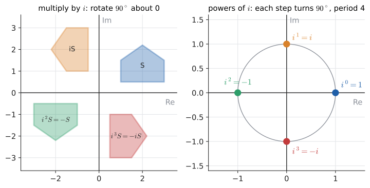
The point \((a, b)\) has moved to \((-b, a)\). That is exactly a rotation by \(90^\circ\) anticlockwise about the origin (try \((1, 0) \to (0, 1) \to (-1, 0) \to (0, -1) \to (1, 0)\)). Now the rule \(i^2 = -1\) has a meaning anyone can see: two quarter-turns make a half-turn. And "the square root of \(-1\)" means "the operation that, done twice, reverses direction".
15.5.3. Why it works in general
Now multiply two general complex numbers. Watch the moduli and arguments in an example: \(z = 2 + i\) and \(w = 1 + i\). Try it: Watch moduli multiply, arguments add.
| modulus | argument | |
|---|---|---|
\(z = 2 + i\) |
\(\sqrt5 \approx 2.236\) |
\(\approx 26.57^\circ\) |
\(w = 1 + i\) |
\(\sqrt2 \approx 1.414\) |
\(45^\circ\) |
\(zw = 1 + 3i\) |
\(\sqrt{10} \approx 3.162\) |
\(\approx 71.57^\circ\) |
The moduli multiplied (\(\sqrt5\cdot\sqrt2 = \sqrt{10}\)) and the arguments added (\(26.57^\circ + 45^\circ = 71.57^\circ\)).
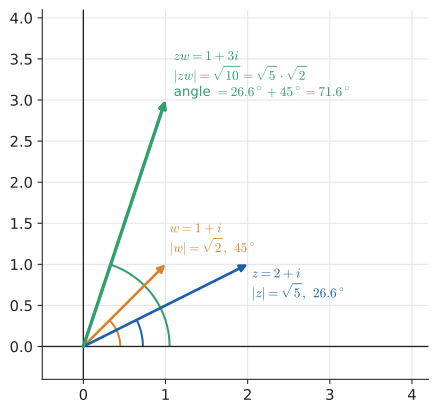
To see that this always happens, write each number using its modulus and argument (from the polar-form picture, \(a = r\cos\theta\), \(b = r\sin\theta\)):
Multiply:
The last step uses the angle-addition formulas from Chapter 13. So:
Multiplying by \(w\) rotates by \(\arg w\) and scales by \(|w|\). Dividing by \(w\) does the reverse: \(|z/w| = |z|/|w|\), \(\arg(z/w) = \arg z - \arg w\).
Read that derivation backwards and something remarkable appears: the angle-addition formulas, which you may once have memorised as arbitrary identities, are nothing more than the real and imaginary parts of "angles add when you multiply". If you forget them, multiply out \((\cos\alpha + i\sin\alpha)(\cos\beta + i\sin\beta)\) and read them off.
15.5.4. Where you’d use this
-
Robotics and navigation: a robot drives 3 m east, turns 60° left and drives 2 m. Each leg is a length times a unit complex number for the heading, so its position is \(3 + 2e^{i\pi/3} = 3 + (1 + \sqrt3\,i) = 4 + 1.732i\): about 4.36 m from the start, in direction \(\arctan(1.732/4) \approx 23.4^\circ\). A turn is a multiplication and a drive is an addition, so a whole route is a short loop. Dead reckoning on ships and wheel odometry on robot vacuums work exactly like this.
-
Graphics: to spin a sprite by 30° every frame, precompute \(w = e^{i\pi/6}\) once and multiply every vertex by \(w\): four real multiplications and two additions per vertex. After 12 frames the sprite is back where it started, because \(w^{12} = e^{2\pi i} = 1\).
15.6. Polar form
The rotation picture suggests describing complex numbers by modulus and argument from the start.
|
Polar form
The polar form (or trigonometric form, or modulus–argument form) of a nonzero complex number is \(z = r(\cos\theta + i\sin\theta)\), where \(r = |z|\) and \(\theta = \arg z\). It is often abbreviated \(r\operatorname{cis}\theta\) ("r cis theta": cos + i sin), and, after the next section, written \(re^{i\theta}\). Conversion: \(a = r\cos\theta\), \(b = r\sin\theta\); \(r = \sqrt{a^2 + b^2}\), \(\theta = \operatorname{atan2}(b, a)\). |
15.6.1. Choosing a form
-
Adding or subtracting? Use rectangular form: add components.
-
Multiplying, dividing, raising to powers, taking roots? Use polar form: multiply moduli, add arguments.
-
Need a final answer as \(a + bi\)? Convert back at the end.
This is the same trade-off as between coordinate systems in geometry: choose the representation in which your operation is simple. Converting has a cost (a square root and an arctangent), so for a single multiplication rectangular form is usually quicker; for \(z^{20}\), polar wins overwhelmingly.
Worked example. Write \(z = 1 + \sqrt3\,i\) in polar form, and convert \(4\operatorname{cis}\frac{2\pi}{3}\) to rectangular form. Try it: Convert 1 + √3 i to polar.
15.7. Euler’s formula
15.7.1. The problem
We found that numbers of the form \(\operatorname{cis}\theta = \cos\theta + i\sin\theta\) obey
Where have you seen a function that turns addition of inputs into multiplication of outputs? The exponential function: \(e^{a}e^{b} = e^{a+b}\) and \(e^0 = 1\) (Chapter 12, Chapter 3). This suggests that \(\operatorname{cis}\theta\) is some kind of exponential of \(\theta\). Which one?
15.7.2. Intuition: three converging arguments
Argument 1 — the law of exponents. As just observed, \(\operatorname{cis}\) satisfies the same law as an exponential.
Argument 2 — rates of change (a preview of Chapter 17). The function \(e^{k\theta}\) has the property that its rate of change is \(k\) times itself. What is the rate of change of \(\operatorname{cis}\theta\) as \(\theta\) increases? The point \(\operatorname{cis}\theta\) moves around the unit circle at unit speed, and its velocity is always perpendicular to its position, pointing anticlockwise — that is, velocity = position rotated by \(90^\circ\) = \(i \times\) position. So \(\operatorname{cis}\theta\) changes at a rate \(i\) times itself, exactly like \(e^{k\theta}\) with \(k = i\). (With derivatives: \(\frac{d}{d\theta}(\cos\theta + i\sin\theta) = -\sin\theta + i\cos\theta = i(\cos\theta + i\sin\theta)\).)
Argument 3 — infinite series (a preview of Taylor series, Chapter 18). The exponential function has a power-series expansion, an "infinite polynomial" in the sense of Chapter 14:
Assume this still makes sense with \(x = i\theta\). Powers of \(i\theta\) cycle through \(1, i, -1, -i\) times powers of \(\theta\):
The two brackets are precisely the power series of \(\cos\theta\) and \(\sin\theta\), as you will see in Chapter 18. All three arguments point to the same conclusion.
15.7.3. Euler’s formula
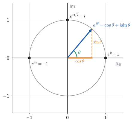
Strictly speaking, this is how we define the exponential of an imaginary number — but it is the only definition consistent with the law of exponents, the rate-of-change property, and the power series all at once, which is why it is universally accepted. Every complex number can now be written compactly as
The multiplication rule is now just the law of exponents.
15.7.4. A numerical check
Trust, but verify. Compare Python’s complex exponential with cosine and sine directly, and sum the power series by hand:
import cmath, math

for theta in [0.0, 0.5, 1.0, math.pi / 2, math.pi]:
    lhs = cmath.exp(1j * theta)
    rhs = complex(math.cos(theta), math.sin(theta))
    print(f"{theta:8.5f}  {lhs:.12f}  {rhs:.12f}")

print(cmath.exp(1j * math.pi) + 1)
0.00000 1.000000000000+0.000000000000j 1.000000000000+0.000000000000j 0.50000 0.877582561890+0.479425538604j 0.877582561890+0.479425538604j 1.00000 0.540302305868+0.841470984808j 0.540302305868+0.841470984808j 1.57080 0.000000000000+1.000000000000j 0.000000000000+1.000000000000j 3.14159 -1.000000000000+0.000000000000j -1.000000000000+0.000000000000j 1.2246467991473532e-16j
import math

def exp_series(z, terms=30):
    total, term = 0, 1
    for n in range(terms):
        total += term
        term = term * z / (n + 1)   # next term: z^(n+1) / (n+1)!
    return total

theta = 1.0
print(exp_series(1j * theta))
print(complex(math.cos(theta), math.sin(theta)))
(0.5403023058681397+0.8414709848078965j) (0.5403023058681398+0.8414709848078965j)
The tiny \(1.22 \times 10^{-16}i\) in the first output is not a flaw in Euler’s formula: math.pi is only the closest double to \(\pi\), and \(\sin\) of that number is about \(1.22 \times 10^{-16}\) (Chapter 32).
|
Euler’s identity
Setting \(\theta = \pi\) gives \(e^{i\pi} = -1\), usually written
\[e^{i\pi} + 1 = 0,\]
linking the five most important constants in mathematics (\(0, 1, e, i, \pi\)) with one each of addition, multiplication, and exponentiation. Geometrically it just says: walking \(\pi\) radians around the unit circle takes you halfway round, to \(-1\). Euler’s formula also yields the startling fact that \(i^i\) is a real number: \(i = e^{i\pi/2}\), so \(i^i = e^{i\cdot i\pi/2} = e^{-\pi/2} \approx 0.2079\). (Complex powers are multi-valued, so this is the principal value.) |
Try it: Walk to e^(iπ) = −1.
|
Euler’s formula explorer
Drag \(\theta\) from 0 to \(2\pi\). Show the point \(e^{i\theta}\) travelling around the unit circle, with its shadow on the real axis tracing \(\cos\theta\) and its shadow on the imaginary axis tracing \(\sin\theta\) as two graphs unrolling beside the circle. A second panel shows the partial sums of the power series \(\sum (i\theta)^n/n!\) as a chain of arrows, each turned \(90^\circ\) from the last and shrinking, spiralling into the point \(e^{i\theta}\). |
15.8. De Moivre’s theorem and powers
15.8.1. The idea
If multiplying by \(z\) rotates by \(\theta\) and scales by \(r\), then multiplying by \(z\) \(n\) times rotates by \(n\theta\) and scales by \(r^n\):
This is De Moivre’s theorem (Abraham de Moivre, 1707). With Euler’s formula it is just the law \((e^{a})^n = e^{na}\).
Input: \(z = a + bi\) and a positive integer \(n\).
Steps:
-
Convert to polar form: \(r = |z|\), \(\theta = \arg z\).
-
Compute \(r^n\) and \(n\theta\).
-
Reduce \(n\theta\) by multiples of \(2\pi\) (optional, but it simplifies the trigonometry).
-
Convert back: \(r^n\cos(n\theta) + i\,r^n\sin(n\theta)\).
Output: \(z^n\) in rectangular form.
15.8.2. Worked examples
\((1 + i)^{10}\). \(r = \sqrt2\), \(\theta = \frac{\pi}{4}\). Try it: Spiral to (1 + i)¹⁰ = 32i.
Alternative method, as a check: \((1 + i)^2 = 1 + 2i + i^2 = 2i\), so \((1 + i)^{10} = (2i)^5 = 32\,i^5 = 32i\) ✓. Repeated squaring is a fine alternative when the base squares to something simple; polar form is the general method. Expanding \((1+i)^{10}\) by the binomial theorem would work too, but would take eleven terms.
\((1 + \sqrt3\,i)^6\). \(r = 2\), \(\theta = \frac{\pi}{3}\), so the result is \(2^6(\cos 2\pi + i\sin 2\pi) = 64\). A complex number whose sixth power is a positive real: it has rotated through exactly one full turn. Try it: See (1 + √3 i)⁶ = 64.
15.8.3. Application: trigonometric identities for free
Expand \((\cos\theta + i\sin\theta)^3\) in two ways. By De Moivre it is \(\cos3\theta + i\sin3\theta\). By the binomial expansion \((c + is)^3 = c^3 + 3c^2(is) + 3c(is)^2 + (is)^3\):
Equate real parts, and use \(\sin^2\theta = 1 - \cos^2\theta\):
Equating imaginary parts similarly gives \(\sin3\theta = 3\sin\theta - 4\sin^3\theta\). Multiple-angle formulas need never be memorised again.
15.9. Roots of unity and nth roots
15.9.1. The problem
How many solutions does \(z^3 = 8\) have? Over the reals, one: \(z = 2\). But polar form lets us run De Moivre backwards. If \(z = re^{i\theta}\) then \(z^3 = r^3e^{3i\theta}\), and we need this to equal \(8 = 8e^{i\cdot0}\). Moduli: \(r^3 = 8\), so \(r = 2\). Arguments: \(3\theta\) must point in the same direction as 0 — but "the same direction" means \(3\theta = 0, 2\pi, 4\pi, \ldots\). So \(\theta = 0, \frac{2\pi}{3}, \frac{4\pi}{3}\) (after that the angles repeat). Three different cube roots: Try it: Plot the cube roots of 8.
Check one: \((-1 + \sqrt3 i)^2 = 1 - 2\sqrt3 i - 3 = -2 - 2\sqrt3 i\), then \((-2 - 2\sqrt3 i)(-1 + \sqrt3 i) = 2 - 2\sqrt3 i + 2\sqrt3 i - 6i^2 = 2 + 6 = 8\) ✓.
|
Roots of unity
The nth roots of unity are the \(n\) complex solutions of \(z^n = 1\): \(\omega^k = e^{2\pi i k/n}\) for \(k = 0, 1, \ldots, n-1\), where \(\omega = e^{2\pi i/n}\) is the primitive nth root of unity (\(\omega\) is the Greek letter omega). They lie on the unit circle at the vertices of a regular \(n\)-gon, one vertex at 1. For \(n \ge 2\) they sum to zero. |
Try it: See the sixth roots of unity.
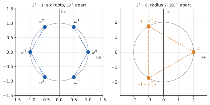
Why do they sum to zero? By symmetry, the regular polygon’s vertices balance around the origin. Algebraically, they form a geometric series (Chapter 14) with ratio \(\omega \ne 1\): Try it: Roots of unity sum to zero.
15.9.2. The method
Input: nonzero \(c\) and a positive integer \(n\).
Steps:
-
Write \(c = Re^{i\phi}\) (modulus \(R\), argument \(\phi\)).
-
The roots all have modulus \(R^{1/n}\) (the ordinary positive real root).
-
Their arguments are \(\dfrac{\phi + 2\pi k}{n}\) for \(k = 0, 1, \ldots, n-1\): start at \(\phi/n\) and step by \(2\pi/n\).
-
Convert each to rectangular form if needed.
Output: the \(n\) distinct nth roots of \(c\), equally spaced on a circle of radius \(R^{1/n}\).
import cmath

def nth_roots(c, n):
    """All n complex nth roots of c."""
    r, phi = cmath.polar(c)
    return [cmath.rect(r ** (1 / n), (phi + 2 * cmath.pi * k) / n)
            for k in range(n)]

for z in nth_roots(8, 3):
    print(f"{z:.6f}", f"{z**3:.6f}")
print(sum(nth_roots(1, 6)))
2.000000+0.000000j 8.000000+0.000000j -1.000000+1.732051j 8.000000-0.000000j -1.000000-1.732051j 8.000000-0.000000j (-1.1102230246251565e-16+4.440892098500626e-16j)
The last line is the sum of the sixth roots of unity: zero, up to rounding.
Worked example. Solve \(z^4 = -16\). Try it: Solve z⁴ = −16 on its circle.
-
\(-16 = 16e^{i\pi}\): \(R = 16\), \(\phi = \pi\).
-
Modulus of each root: \(16^{1/4} = 2\).
-
Arguments: \(\frac{\pi + 2\pi k}{4}\) for \(k = 0, 1, 2, 3\): \(\frac{\pi}{4}, \frac{3\pi}{4}, \frac{5\pi}{4}, \frac{7\pi}{4}\).
-
Rectangular: \(2e^{i\pi/4} = 2\left(\frac{\sqrt2}{2} + \frac{\sqrt2}{2}i\right) = \sqrt2 + \sqrt2 i\), and similarly the others: the four roots are \(\pm\sqrt2 \pm \sqrt2\,i\) (all four sign combinations).
|
The principal root is a convention
Calculators and |
15.9.3. Where you’d use this
-
Mains electricity (three-phase power): power stations generate three voltages of the same size, a third of a cycle apart. As phasors they are \(V_0\), \(V_0\,\omega^{-1}\) and \(V_0\,\omega^{-2}\) with \(\omega = e^{2\pi i/3}\): the three cube roots of unity, scaled. Because the cube roots of unity sum to zero, the three voltages add to zero at every instant. With a balanced load, the currents returning through the shared neutral wire cancel too, so it can be thin or omitted. That saving in copper is why grids worldwide are three-phase. In the UK each phase is 230 V (325 V peak) at 50 Hz. Try it: Watch three-phase phasors cancel.
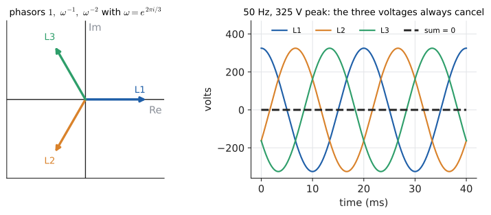 Figure 131. Three-phase mains. Left: the three phasors are the cube roots of unity (scaled), and they sum to zero. Right: the three 50 Hz voltages, and their sum, which is zero at every instant.
-
Graphics: the vertices of a regular \(n\)-gon of radius \(r\) centred at \(c\) are \(c + r\omega^k\) for \(k = 0, \ldots, n - 1\). For a hexagonal map tile of radius 10 at \((50, 50)\), that gives \((60, 50), (55, 58.66), (45, 58.66), (40, 50), (45, 41.34), (55, 41.34)\). Strategy games with hex grids generate their tiles this way, in one line of code.
-
Signal processing: the FFT below is roots of unity at industrial scale.
15.10. The fundamental theorem of algebra
15.10.1. Every polynomial has a root
We extended the reals to solve one equation, \(x^2 + 1 = 0\). A natural worry: will \(x^2 = i\) or \(x^5 + ix + 3 = 0\) force yet another extension? The answer, and the reason complex numbers are the end of this road, is one of the great theorems of mathematics.
|
Fundamental theorem of algebra
Fundamental theorem of algebra: every polynomial of degree \(n \ge 1\) with complex coefficients has at least one complex root. Consequently it factors completely into \(n\) linear factors,
\[p(z) = a_n(z - z_1)(z - z_2)\cdots(z - z_n),\]
so it has exactly \(n\) roots in \(\mathbb{C}\), counted with multiplicity (a repeated factor like \((z - 2)^2\) counts twice). A number system in which every polynomial has a root is called algebraically closed. |
The "consequently" is the factor theorem from Chapter 7: if \(z_1\) is a root, then \((z - z_1)\) is a factor, and the remaining quotient has degree \(n - 1\), which again has a root, and so on.
The proofs (Gauss gave several, starting in 1799) need tools beyond this book, but here is the intuition. For a huge circle \(|z| = R\), the polynomial behaves like its leading term \(z^n\), which winds around the origin \(n\) times as \(z\) goes once around the circle. For a tiny circle, \(p(z)\) stays close to \(p(0)\) and does not wind around the origin at all (if \(p(0) \ne 0\)). Shrinking the circle continuously from large to small, the image loop must at some point pass through the origin — and that is a root.
15.10.2. Complex roots of real quadratics
For a quadratic with real coefficients and negative discriminant, the quadratic formula (Chapter 8) now simply works:
Worked example. Solve \(x^2 - 4x + 13 = 0\). Try it: See the roots 2 ± 3i.
Check: \((2 + 3i)^2 - 4(2 + 3i) + 13 = (4 + 12i - 9) - 8 - 12i + 13 = 0\) ✓.
Alternative: completing the square. \(x^2 - 4x + 13 = (x - 2)^2 + 9 = 0\), so \((x - 2)^2 = -9\), \(x - 2 = \pm3i\), \(x = 2 \pm 3i\). Same answer, and it shows the geometry: the vertex of the parabola is at \((2, 9)\), above the axis; the real part of the roots is the axis of symmetry, and the imaginary part measures how far the parabola "misses" the x-axis.
import cmath

def solve_quadratic(a, b, c):
    """Both roots of ax^2 + bx + c = 0, complex if necessary."""
    disc = b * b - 4 * a * c
    root = cmath.sqrt(disc)          # works for negative disc too
    return (-b + root) / (2 * a), (-b - root) / (2 * a)

print(solve_quadratic(1, -4, 13))
print(solve_quadratic(1, -5, 6))
print(solve_quadratic(1, 0, 1))
((2+3j), (2-3j)) ((3+0j), (2+0j)) (1j, -1j)
15.10.3. Conjugate pairs
Notice the roots came as \(2 + 3i\) and \(2 - 3i\), a conjugate pair. That is no accident. If a polynomial has real coefficients and \(p(z) = 0\), conjugate everything: since conjugation respects sums and products and leaves real coefficients alone, \(p(\bar z) = \overline{p(z)} = \bar 0 = 0\). So non-real roots of real polynomials come in conjugate pairs. Consequences:
-
A real cubic (odd degree) must have at least one real root — non-real roots pair up, and three cannot all pair.
-
Multiplying a conjugate pair of factors gives a real quadratic: \((x - (2 + 3i))(x - (2 - 3i)) = (x - 2)^2 + 9 = x^2 - 4x + 13\). So every real polynomial factors into real linear and real irreducible quadratic factors — a fact used in partial fractions for integration (Chapter 19).
Example. \(x^3 - 1 = (x - 1)(x^2 + x + 1)\). The quadratic has discriminant \(1 - 4 = -3\), so roots \(\frac{-1 \pm \sqrt3 i}{2}\). Together with 1 these are the three cube roots of unity, \(e^{0}, e^{2\pi i/3}, e^{4\pi i/3}\) — the algebra and the geometry agree.
15.10.4. Where you’d use this
-
Car suspension and earthquake-proof buildings: a car’s suspension is a mass on a spring with a damper. Its motion \(x(t)\) satisfies a differential equation whose behaviour is set by the roots of a quadratic, its characteristic equation (deriving it needs the derivatives of Chapter 17 and a little more). For a typical setting, that quadratic might be \(r^2 + 2r + 26 = 0\), with roots \(r = -1 \pm 5i\). The real part \(-1\) says the bounce dies away like \(e^{-t}\). The imaginary part 5 says it oscillates at 5 rad/s, a period of \(2\pi/5 \approx 1.26\) s. If the damper wears out, the real part moves towards 0 and the car keeps bouncing. Engineers tune the damper so the roots sit where the ride is comfortable. Try it: Plot the suspension roots.
-
Control and computing: the same rule decides whether an autopilot, a drone’s stabiliser or a digital audio filter is stable. Find the roots (the poles) of its characteristic polynomial and check they are on the safe side: negative real part for continuous systems, inside the unit circle for digital ones.
numpy.rootsand the conjugate-pair rule do the work.
15.11. Applications
15.11.1. Electrical engineering: AC circuits
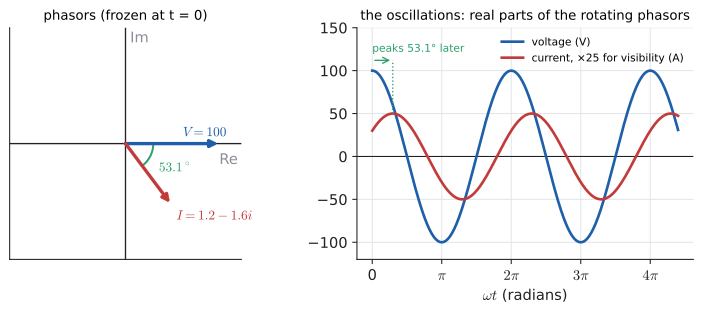
In alternating-current circuits, voltages and currents oscillate sinusoidally, \(V(t) = V_0\cos(\omega t + \phi)\) (here \(\omega\) is the angular frequency, not a root of unity). Resistors, capacitors, and inductors each respond differently: a resistor’s current is in step with the voltage; an inductor’s current lags by a quarter cycle; a capacitor’s leads by a quarter cycle. Tracking these phase shifts with trigonometric identities is miserable.
Engineers instead represent each oscillation by a complex number, its phasor \(V_0e^{i\phi}\) (the oscillation is the real part of \(V_0e^{i\phi}e^{i\omega t}\)). A "quarter-cycle shift" is multiplication by \(\pm i\) — the quarter-turn again. Each component gets a complex impedance (generalised resistance):
and Ohm’s law \(V = IZ\) works with complex numbers. Components in series add their impedances; in parallel, the reciprocals add — exactly as for plain resistors.
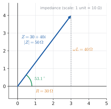
Worked example. A 30 Ω resistor in series with an inductor of reactance \(\omega L = 40\) Ω is driven by a voltage of amplitude 100 V. Then \(Z = 30 + 40i\) Ω, and Try it: Solve the AC circuit with phasors.
The current’s amplitude is \(|I| = \sqrt{1.44 + 2.56} = 2\) A (equivalently \(100/|Z| = 100/50\)), and its phase is \(\arg I = -\arctan\frac{1.6}{1.2} \approx -53.1^\circ\): it lags the voltage by \(53.1^\circ\). One complex division replaced a page of trigonometry.
15.11.2. Signal processing
Any reasonable periodic signal is a sum of sines and cosines (Fourier series), and Euler’s formula packs each cosine–sine pair into one complex exponential: \(\cos\omega t = \frac{e^{i\omega t} + e^{-i\omega t}}{2}\). Filtering a signal (removing hiss, isolating a radio station, equalising audio) becomes multiplying each frequency component by a complex number that scales its amplitude and shifts its phase. The DFT and FFT from the sidebar above are the computational form.
15.11.3. Quantum mechanics (an aside)
In quantum mechanics, complex numbers are not a convenience but part of the foundations. The state of a system is described by complex amplitudes; the probability of an outcome is the squared modulus \(|\psi|^2\) of its amplitude. Because amplitudes have phases, two paths to the same outcome can cancel (destructive interference) or reinforce, which is what the double-slit experiment shows. Schrödinger’s equation, \(i\hbar\frac{\partial\psi}{\partial t} = \hat H\psi\), has \(i\) right at the front. Quantum computing algorithms (including Shor’s factoring algorithm, which uses a quantum Fourier transform built from roots of unity) are manipulations of these complex amplitudes.
15.11.4. Elsewhere
-
Fluid flow and aerodynamics: complex functions map simple flows (around a cylinder) to complicated ones (around an aerofoil) — the Joukowski transform.
-
Control engineering: a system is stable when the roots of its characteristic polynomial (often complex) have negative real parts.
-
Linear algebra: a rotation matrix has no real eigenvectors (nothing stays on its own line when you rotate), but it has complex eigenvalues \(e^{\pm i\theta}\) (Chapter 28).
15.12. The Mandelbrot set
The most famous picture in mathematics comes from iterating one tiny complex formula.
15.12.1. The problem
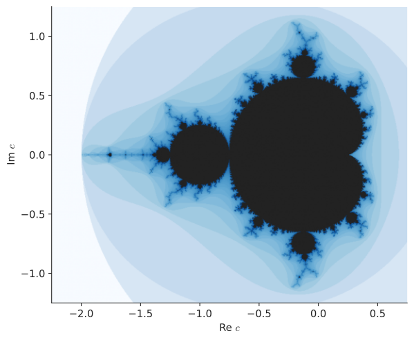
Pick a complex number \(c\). Start with \(z_0 = 0\) and repeatedly apply \(z_{n+1} = z_n^2 + c\) (a recurrence, Chapter 14). Does the sequence stay bounded, or does it run off to infinity? The Mandelbrot set is the set of all \(c\) for which it stays bounded.
Try a few by hand: Try it: Follow the orbit of c = i.
-
\(c = 1\): \(0, 1, 2, 5, 26, 677, \ldots\) — escapes. Not in the set.
-
\(c = -1\): \(0, -1, 0, -1, 0, \ldots\) — a cycle. In the set.
-
\(c = i\): \(0,\ i,\ i^2 + i = -1 + i,\ (-1 + i)^2 + i = -2i + i = -i,\ (-i)^2 + i = -1 + i, \ldots\) — cycles between \(-1 + i\) and \(-i\). In the set.
A useful fact makes computation possible: once \(|z_n| > 2\), the sequence is guaranteed to escape to infinity. (Roughly: when \(|c| \le 2\) and \(|z| > 2\), squaring makes \(|z|\) grow faster than adding \(c\) can pull it back; and if \(|c| > 2\) the very first step already exceeds 2.) So we iterate until \(|z| > 2\) or until we give up after some maximum number of steps.
Input: a complex number \(c\); an iteration limit \(N\) (say 50–1000).
Steps:
-
Set \(z \leftarrow 0\).
-
For \(n = 0, 1, \ldots, N-1\):
-
Update \(z \leftarrow z^2 + c\).
-
If \(|z| > 2\), stop: \(c\) is outside the set; report the escape step \(n\).
-
-
If the loop finishes without escaping, report \(c\) as (probably) inside the set.
Output: inside / outside, and for outside points the escape step, which is used to choose a colour.
To draw the set, run this for the \(c\) at the centre of every pixel.
def escape_count(c, max_iter=50):
    """Iterate z -> z^2 + c from z = 0; return the step at which |z| > 2,
    or max_iter if it never escapes (c is then taken to be in the set)."""
    z = 0j
    for n in range(max_iter):
        z = z * z + c
        if abs(z) > 2:
            return n
    return max_iter

def mandelbrot_ascii(width=64, height=20, max_iter=50):
    shades = " .:-=+*"              # outside: escapes fast ... escapes slowly
    lines = []
    for row in range(height):
        y = 1.2 - 2.4 * row / (height - 1)
        line = ""
        for col in range(width):
            x = -2.1 + 2.7 * col / (width - 1)
            n = escape_count(complex(x, y), max_iter)
            if n == max_iter:
                line += "#"             # inside the set
            else:
                line += shades[min(n // 2, len(shades) - 1)]
        lines.append(line)
    return "\n".join(lines)

print(mandelbrot_ascii())
..............................
.........................::-*:::..........
...........................::::-=+*=-::..........
...........................::::-=*####**=:::::........
........................:::=-+--===*#####*===-::-=:.....
..................:::::::::--=*#################*##*#::...
.............:-::::::::::---*#*#####################*--::..
..........:::::-***++**+====+*#########################+-:..
........::::::--+**#########*##########################*=::..
.::::--::---=+*#*#####################################*-:::..
.::::--::---=+*#*#####################################*-:::..
........::::::--+**#########*##########################*=::..
..........:::::-***++**+====+*#########################+-:..
.............:-::::::::::---*#*#####################*--::..
..................:::::::::--=*#################*##*#::...
........................:::=-+--===*#####*===-::-=:.....
...........................::::-=*####**=:::::........
...........................::::-=+*=-::..........
.........................::-*:::..........
..............................
|
Where the failure modes hide
The escape-time test can only ever prove that a point is outside. A point that has not escaped after \(N\) steps might escape at step \(N + 1\); near the boundary, points can take millions of iterations. Raising \(N\) sharpens the picture but costs time, and deep zooms eventually run out of double-precision accuracy (pixels closer together than about \(10^{-16}\) times the coordinates are indistinguishable), which is why deep-zoom renderers use arbitrary precision or clever perturbation methods (Chapter 32). |
Try it: Zoom past double precision.
|
Iteration, chaos, and beauty
Benoit Mandelbrot produced the first crude printouts of the set at IBM in 1980. Its boundary is a fractal: zoom in anywhere and new detail appears forever, including tiny distorted copies of the whole set. Its area is still not known exactly (about 1.506). Mandelbrot coined the word fractal from the Latin fractus, broken. A deep theorem says the set is connected — all one piece — even though the thin filaments make it look like scattered islands in any finite picture. |
|
Explore the Mandelbrot set
Click any point \(c\) in the plane and watch the orbit \(0, c, c^2 + c, \ldots\) drawn as a path of connected dots: spiralling into a fixed point, cycling, or flying off. Zoom into the boundary with a scroll wheel and a slider for the iteration limit, and see where double precision gives out. Try it: Explore the Mandelbrot set |
|
Multiply and watch
Draw a shape (a letter F works well, since it has no symmetry). Drag a complex number \(w\) around the plane and watch the shape multiplied by \(w\) update live: rotating as \(w\) moves around a circle, growing and shrinking as \(w\) moves in and out, and turning exactly a quarter-turn when \(w = i\). A second mode shows \(z \mapsto z^2\) distorting a grid, doubling all angles. Try it: Multiply and watch |
15.13. Interactive tools
Browser tools on the companion website that go with this chapter. Each example link in the chapter opens one of them with that example already set up.
15.14. Exercises
Recognition
-
Give the real and imaginary parts of: (a) \(7 - 2i\) (b) \(5i\) (c) \(-3\) (d) \(\frac{1 + i}{2}\).
-
Simplify \(i^{2026}\), \(i^{-1}\), and \(i^{4k+3}\) for an integer \(k\).
-
Describe, in words, the effect on the complex plane of multiplying every point by: (a) 3 (b) \(-1\) (c) \(i\) (d) \(-i\) (e) \(1 + i\).
Application
-
Compute in the form \(a + bi\): (a) \((2 + 3i)(4 - i)\) (b) \((3 - 2i)^2\) (c) \(\dfrac{5 - i}{2 + 3i}\).
-
Find the modulus and principal argument of (a) \(-2 + 2i\) (b) \(-\sqrt3 - i\) (c) \(-4\).
-
Use De Moivre’s theorem to compute \((-1 + i)^8\). Check by repeated squaring.
-
Solve (a) \(x^2 + 6x + 13 = 0\) (b) \(z^4 = -16\) (c) \(z^3 = -8i\).
-
Rotate the point \((4, 1)\) by \(90^\circ\) anticlockwise about the point \((1, 1)\) using complex multiplication.
Problem solving
-
Show that \(|z|^2 = z\bar z\) and use it to prove \(|zw| = |z||w|\) without polar form.
-
Use De Moivre’s theorem to express \(\cos 4\theta\) in terms of \(\cos\theta\).
-
A cubic with real coefficients has roots \(3\) and \(1 - 2i\). Find its third root and write the cubic (leading coefficient 1) with real coefficients.
-
Decide by iterating whether \(c = 0.5\) and \(c = -i\) are in the Mandelbrot set.
Answers
-
(a) Re = 7, Im = \(-2\). (b) Re = 0, Im = 5. (c) Re = \(-3\), Im = 0. (d) Re = \(\tfrac12\), Im = \(\tfrac12\).
-
\(2026 = 4\cdot506 + 2\), so \(i^{2026} = i^2 = -1\). \(i^{-1} = \frac{1}{i} = \frac{i}{i^2} = -i\). \(i^{4k+3} = (i^4)^k i^3 = -i\).
-
(a) Stretch away from 0 by a factor 3. (b) Rotate \(180^\circ\) (point reflection through 0). (c) Rotate \(90^\circ\) anticlockwise. (d) Rotate \(90^\circ\) clockwise. (e) \(|1 + i| = \sqrt2\), \(\arg = 45^\circ\): rotate \(45^\circ\) anticlockwise and scale by \(\sqrt2\).
-
(a) \(8 - 2i + 12i - 3i^2 = 11 + 10i\). (b) \(9 - 12i + 4i^2 = 5 - 12i\). (c) \(\frac{(5 - i)(2 - 3i)}{4 + 9} = \frac{10 - 15i - 2i + 3i^2}{13} = \frac{7 - 17i}{13} = \frac{7}{13} - \frac{17}{13}i\).
-
(a) \(|z| = \sqrt{8} = 2\sqrt2\); second quadrant, reference angle \(\frac{\pi}{4}\), so \(\arg = \frac{3\pi}{4}\) (\(135^\circ\)). (b) \(|z| = \sqrt{3 + 1} = 2\); third quadrant, reference angle \(\arctan\frac{1}{\sqrt3} = \frac{\pi}{6}\), so \(\arg = -(\pi - \frac{\pi}{6}) = -\frac{5\pi}{6}\) (\(-150^\circ\)). (c) \(|z| = 4\), \(\arg = \pi\).
-
\(-1 + i = \sqrt2\,e^{3\pi i/4}\). \((-1 + i)^8 = (\sqrt2)^8 e^{6\pi i} = 16\,e^{0} = 16\). Check: \((-1 + i)^2 = 1 - 2i - 1 = -2i\); \((-2i)^2 = -4\); \((-4)^2 = 16\) ✓.
-
(a) \(x = \frac{-6 \pm \sqrt{36 - 52}}{2} = \frac{-6 \pm 4i}{2} = -3 \pm 2i\). (b) \(\pm\sqrt2 \pm \sqrt2\,i\) (worked in the text). (c) \(-8i = 8e^{-i\pi/2}\): modulus of roots 2, arguments \(\frac{-\pi/2 + 2\pi k}{3} = -\frac{\pi}{6}, \frac{\pi}{2}, \frac{7\pi}{6}\). Roots: \(2e^{-i\pi/6} = \sqrt3 - i\), \(2e^{i\pi/2} = 2i\), \(2e^{7i\pi/6} = -\sqrt3 - i\). Check: \((2i)^3 = 8i^3 = -8i\) ✓.
-
\(p = 4 + i\), \(c = 1 + i\). \(p - c = 3\); times \(i\): \(3i\); plus \(c\): \(1 + 4i\). The image is \((1, 4)\).
-
With \(z = a + bi\): \(z\bar z = a^2 - (bi)^2 = a^2 + b^2 = |z|^2\). Then \(|zw|^2 = (zw)\overline{(zw)} = zw\,\bar z\,\bar w = (z\bar z)(w\bar w) = |z|^2|w|^2\); take non-negative square roots.
-
Real part of \((c + is)^4 = c^4 + 4c^3(is) + 6c^2(is)^2 + 4c(is)^3 + (is)^4\) is \(c^4 - 6c^2s^2 + s^4\). Substitute \(s^2 = 1 - c^2\): \(c^4 - 6c^2(1 - c^2) + (1 - c^2)^2 = c^4 - 6c^2 + 6c^4 + 1 - 2c^2 + c^4 = 8c^4 - 8c^2 + 1\). So \(\cos4\theta = 8\cos^4\theta - 8\cos^2\theta + 1\). (Check \(\theta = 0\): \(8 - 8 + 1 = 1\) ✓.)
-
Real coefficients, so \(1 + 2i\) is also a root. \((x - (1 - 2i))(x - (1 + 2i)) = (x - 1)^2 + 4 = x^2 - 2x + 5\). The cubic is \((x - 3)(x^2 - 2x + 5) = x^3 - 5x^2 + 11x - 15\).
-
\(c = 0.5\): \(0, 0.5, 0.75, 1.0625, 1.6289, 3.1533\) — exceeds 2, escapes: not in the set. \(c = -i\): \(0, -i, (-i)^2 - i = -1 - i, (-1 - i)^2 - i = 2i - i = i, i^2 - i = -1 - i, \ldots\) — cycles between \(-1 - i\) and \(i\): bounded, in the set.
15.15. Mastery check
-
Compute \((3 - 2i)^2\) and its modulus.
-
Write \(\dfrac{4 + 2i}{1 - i}\) in the form \(a + bi\).
-
Write \(1 - \sqrt3\,i\) in polar (exponential) form, then compute \((1 - \sqrt3\,i)^5\) in rectangular form.
-
Find all three cube roots of \(-8i\) and sketch them.
-
Solve \(x^2 - 2x + 10 = 0\) and check one root by substitution.
-
Explain, in a sentence, why multiplying by \(i\) twice is the same as multiplying by \(-1\), in terms of geometry.
-
Use Euler’s formula to write \(e^{i\pi/3}\) in the form \(a + bi\), and explain why \(|e^{i\theta}| = 1\) for every real \(\theta\).
Decision rule: All correct without hesitation → move on to Chapter 16. Stuck on 1–2 → reread Section 15.2 and Section 15.4. Stuck on 3–4 → reread Section 15.5, Section 15.6, and Section 15.9. Stuck on 6–7 → revisit Section 15.5 and Section 15.7 with the diagrams, then the exercises.
Mastery check answers
-
\((3 - 2i)^2 = 9 - 12i + 4i^2 = 5 - 12i\); \(|5 - 12i| = \sqrt{25 + 144} = 13\) (equivalently \(|3 - 2i|^2 = 13\)).
-
\(\frac{(4 + 2i)(1 + i)}{(1 - i)(1 + i)} = \frac{4 + 4i + 2i + 2i^2}{2} = \frac{2 + 6i}{2} = 1 + 3i\). Check: \((1 + 3i)(1 - i) = 1 - i + 3i - 3i^2 = 4 + 2i\) ✓.
-
\(|1 - \sqrt3 i| = 2\); fourth quadrant, reference angle \(\frac{\pi}{3}\), so \(1 - \sqrt3 i = 2e^{-i\pi/3}\). Then \((2e^{-i\pi/3})^5 = 32e^{-5i\pi/3} = 32e^{i\pi/3}\) (add \(2\pi\)) \(= 32\left(\frac12 + \frac{\sqrt3}{2}i\right) = 16 + 16\sqrt3\,i\).
-
\(-8i = 8e^{-i\pi/2}\); roots \(\sqrt3 - i\), \(2i\), \(-\sqrt3 - i\), on a circle of radius 2, \(120^\circ\) apart (an equilateral triangle with a vertex at \(2i\)).
-
\(x = \frac{2 \pm \sqrt{4 - 40}}{2} = \frac{2 \pm 6i}{2} = 1 \pm 3i\). Check \(1 + 3i\): \((1 + 3i)^2 - 2(1 + 3i) + 10 = (1 + 6i - 9) - 2 - 6i + 10 = 0\) ✓.
-
Multiplying by \(i\) rotates the plane a quarter-turn about 0; two quarter-turns make a half-turn, which sends every point \(z\) to \(-z\) — the same as multiplying by \(-1\). That is what \(i^2 = -1\) means.
-
\(e^{i\pi/3} = \cos\frac{\pi}{3} + i\sin\frac{\pi}{3} = \frac12 + \frac{\sqrt3}{2}i\). \(|e^{i\theta}| = \sqrt{\cos^2\theta + \sin^2\theta} = 1\) by the Pythagorean identity: every \(e^{i\theta}\) lies on the unit circle.