A game needs to rotate a spaceship sprite by 30°. A photo editor needs to skew an image so a slanted building looks upright. A 3D engine must take every vertex of a model, place it in a world, look at it from a camera, and flatten the result onto a screen, 60 times a second, for millions of vertices. A neural network must turn a 768-number embedding into a 3072-number hidden representation.

Each of these is a function that takes vectors in and produces vectors out. We want a representation of such functions that is compact, fast to apply, easy to combine, and easy to reverse. For a very important class of them, the linear transformations, that representation is the matrix.

The best way to understand a transformation of the plane is to apply it to everything at once and watch what happens to the coordinate grid. Here are six transformations applied to the grid, to an asymmetric letter F (so you can see flips and turns), and to the two standard basis vectors \(\mathbf{e}_1 = (1, 0)\) (green) and \(\mathbf{e}_2 = (0, 1)\) (red).

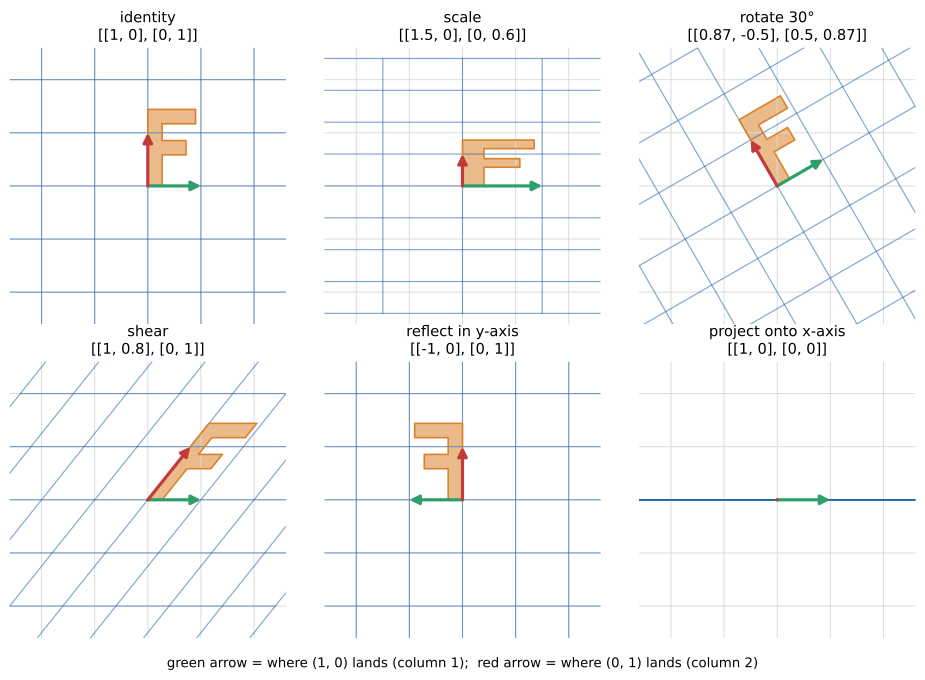
Look at what all six have in common:

These are the visual signatures of a linear transformation. A rotation keeps squares as squares; a scale stretches them into rectangles; a shear slants them into parallelograms; a reflection flips the F; a projection flattens the whole plane onto a line. But in every case, a regular grid becomes a regular grid (possibly a flattened one).

The pictures have a precise algebraic meaning. A function \(T\) from vectors to vectors is linear if, for all vectors \(\mathbf{u}, \mathbf{v}\) and scalars \(c\),

In words: transforming a sum gives the sum of the transforms, and transforming a scaled vector gives the scaled transform. Tip-to-tail parallelograms map to tip-to-tail parallelograms. Taking \(c = 0\) shows \(T(\mathbf{0}) = \mathbf{0}\): the origin is fixed. And "evenly spaced lines stay evenly spaced" is the second rule applied to the multiples \(1\mathbf{v}, 2\mathbf{v}, 3\mathbf{v}, \ldots\).

Rotations, scalings, shears, reflections and projections through the origin are all linear. Some important transformations are not: translation (sliding everything by a fixed vector) moves the origin, so it fails the test. We’ll rescue translation with a clever trick in Section 27.11.

A linear transformation acts on infinitely many vectors. How can a finite list of numbers possibly describe it?

Every vector in the plane is a combination of the basis vectors: \((x, y) = x\,\mathbf{e}_1 + y\,\mathbf{e}_2\). Linearity says a transformation respects combinations. So

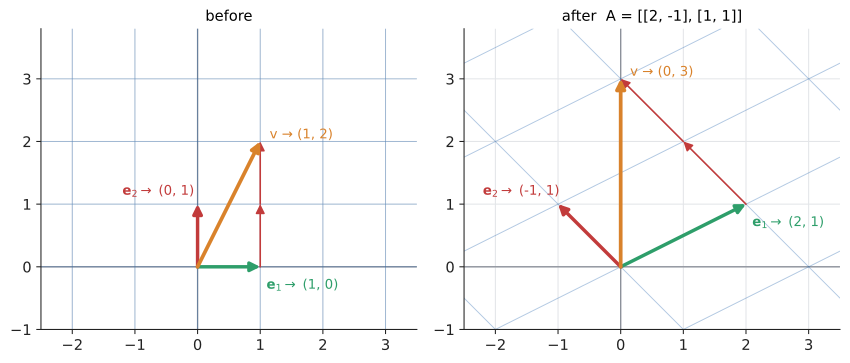
That’s the whole secret. Once you know where \(\mathbf{e}_1\) and \(\mathbf{e}_2\) land, you know where everything lands. A linear transformation of the plane is completely determined by two vectors, four numbers. Write those two landing spots side by side as columns, and you have the matrix:

Applying a matrix to a vector is written \(A\mathbf{x}\), and from the derivation above we already know what it must be: a linear combination of the columns, weighted by the entries of \(\mathbf{x}\).

Now read the final result row by row. The top entry \(ax + by\) is the dot product of the first row \((a, b)\) with \(\mathbf{x}\); the bottom entry is the dot product of the second row with \(\mathbf{x}\). So there are two equally correct ways to compute \(A\mathbf{x}\):

Try it: Step through matrix × vector.

Compute \(A\mathbf{v}\) for \(A = \begin{bmatrix} 2 & -1 \\ 1 & 1 \end{bmatrix}\) and \(\mathbf{v} = (1, 2)\), both ways.

Same answer, of course, and it matches the diagram. In code the two views are two loop orders over the same arithmetic:

The column view lets you read a matrix geometrically. Faced with \(\begin{bmatrix} 1 & 0.8 \\ 0 & 1 \end{bmatrix}\), don’t see four numbers: see "\(\mathbf{e}_1\) stays at \((1, 0)\); \(\mathbf{e}_2\) tips over to \((0.8, 1)\)". That’s a horizontal shear: points slide sideways by an amount proportional to their height. Faced with \(\begin{bmatrix} 1 & 0 \\ 0 & 0 \end{bmatrix}\): "\(\mathbf{e}_1\) stays, \(\mathbf{e}_2\) is crushed to zero", a projection onto the x-axis.

A matrix–vector product is the right tool whenever several totals each depend on the same list of inputs.

Stretch horizontally by \(s_x\) and vertically by \(s_y\): \(\mathbf{e}_1 \mapsto (s_x, 0)\), \(\mathbf{e}_2 \mapsto (0, s_y)\).

A matrix that’s zero off the main diagonal (top-left to bottom-right) is a diagonal matrix, and it just scales each axis independently. Diagonal matrices are the simplest matrices there are, and much of Chapter 28 is about turning other matrices into diagonal ones.

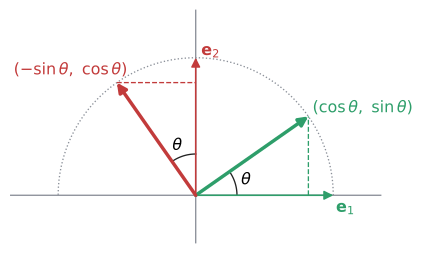
Rotate the plane anticlockwise by angle \(\theta\) about the origin. Where does \(\mathbf{e}_1 = (1, 0)\) go? It’s a unit vector, so it stays on the unit circle, now at angle \(\theta\): by the definition of sine and cosine (Chapter 13), it lands at \((\cos\theta, \sin\theta)\).

Where does \(\mathbf{e}_2 = (0, 1)\) go? It starts at angle \(90^\circ\) and ends at \(90^\circ + \theta\), so it lands at \((\cos(90^\circ + \theta), \sin(90^\circ + \theta)) = (-\sin\theta, \cos\theta)\). (You can also see this from the diagram: the rotated \(\mathbf{e}_2\) is the rotated \(\mathbf{e}_1\) turned a further quarter-turn, and a quarter-turn sends \((p, q)\) to \((-q, p)\).)

Put the landing spots in as columns:

This is the formula behind every 2D rotation in every game engine, and it falls out of nothing more than "columns are where the basis vectors go" plus the unit circle. Worked check: rotate \((3, 4)\) by \(90^\circ\). With \(\cos 90^\circ = 0\), \(\sin 90^\circ = 1\): \((3\cdot 0 - 4\cdot 1,\ 3\cdot 1 + 4\cdot 0) = (-4, 3)\). Its length is still 5, and \((3, 4)\cdot(-4, 3) = -12 + 12 = 0\), so it’s perpendicular to the original. ✓

A game rotates a sprite by \(90^\circ\) and then shears it. With a million vertices, you’d rather not apply two matrices to every vertex; you’d like one matrix that does both. What is it? And does the order matter?

Let \(B\) be the first transformation and \(A\) the second. The combined transformation sends \(\mathbf{x}\) to \(A(B\mathbf{x})\). Doing one linear transformation after another is still linear (grid lines stay straight through both steps), so it has a matrix, and we find it as always: by tracking the basis vectors.

So the combined matrix, written \(AB\), has columns \(A\mathbf{b}_1\) and \(A\mathbf{b}_2\):

Each column of the product is \(A\) times the corresponding column of \(B\). That’s the definition of matrix multiplication, and it is forced by the requirement that \((AB)\mathbf{x} = A(B\mathbf{x})\).

Now apply the row view of matrix–vector multiplication to each \(A\mathbf{b}_j\): entry \(i\) of column \(j\) is (row \(i\) of \(A\)) \(\cdot\) (column \(j\) of \(B\)). That’s the familiar "row times column" rule:

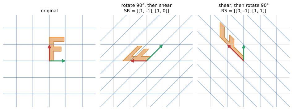
Let \(R = \begin{bmatrix} 0 & -1 \\ 1 & 0 \end{bmatrix}\) (rotate \(90^\circ\)) and \(S = \begin{bmatrix} 1 & 1 \\ 0 & 1 \end{bmatrix}\) (shear). Compute both orders.

\(SR\) (rotate first, then shear). Columns of \(R\) are \((0, 1)\) and \((-1, 0)\). Apply \(S\) to each:

\(RS\) (shear first, then rotate). Columns of \(S\) are \((1, 0)\) and \((1, 1)\):

\(SR \neq RS\). The picture makes it obvious:

Think of everyday actions: "put on socks, then shoes" differs from "shoes, then socks". Some pairs do commute (two rotations about the same point; two scalings; anything with the identity), but you may never assume it.

Try it: Multiply row by column, stepped.

Compute \(\begin{bmatrix} 1 & 2 \\ 3 & 4 \end{bmatrix}\begin{bmatrix} 5 & 6 \\ 7 & 8 \end{bmatrix}\). Try it: Step through this product.

so the product is \(\begin{bmatrix} 19 & 22 \\ 43 & 50 \end{bmatrix}\). (In the other order you’d get \(\begin{bmatrix} 23 & 34 \\ 31 & 46 \end{bmatrix}\): different again.) Try it: Try the other order.

The identity matrix \(I\) has 1s on the diagonal and 0s elsewhere. It sends every basis vector to itself, so it’s the "do nothing" transformation: \(AI = IA = A\). It plays the role of 1 in ordinary multiplication.

Matrix multiplication is associative: \((AB)C = A(BC)\). Both sides mean "do \(C\), then \(B\), then \(A\)", so they must be the same transformation. This is why a graphics engine can pre-multiply a chain of a dozen transformations into a single matrix once per frame and then apply that one matrix to every vertex. It’s also why \(A^n\) (\(A\) multiplied by itself \(n\) times, "apply \(A\) \(n\) times") is unambiguous, which Chapter 28 exploits heavily.

Three nested loops of length \(n\) mean \(n^3\) multiplications for two \(n\times n\) matrices: \(O(n^3)\). Doubling \(n\) multiplies the work by 8. For \(n = 1000\) that’s a billion multiply-adds: a minute or more in pure Python, a few tens of milliseconds in NumPy.

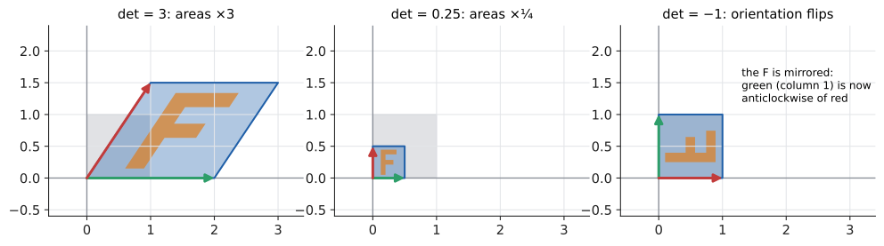
When a matrix transforms the plane, the unit square (the square spanned by \(\mathbf{e}_1\) and \(\mathbf{e}_2\)) becomes a parallelogram spanned by the two columns. How does its area change? And can we tell from the numbers alone whether the transformation flips space over, or flattens it completely?

Because grid lines stay parallel and evenly spaced, every grid square becomes a copy of the same parallelogram. So every region’s area is multiplied by the same factor: the area of the transformed unit square. That factor, with a sign attached to record whether the transformation flips orientation, is the determinant, \(\det A\).

Let \(A = \begin{bmatrix} a & b \\ c & d \end{bmatrix}\) with all entries positive and the columns \((a, c)\) and \((b, d)\) arranged as in the first panel above. The parallelogram fits in a rectangle of width \(a + b\) and height \(c + d\). The parts of the rectangle outside the parallelogram are two triangles of area \(\tfrac{1}{2}ac\), two of area \(\tfrac{1}{2}bd\), and two small rectangles of area \(bc\). Subtract them:

(Sketching that rectangle and its six pieces on paper is well worth the minute it takes.) In general,

and the sign comes out right automatically: swapping the columns (which mirrors the picture) gives \(bc - ad\), the negative. Notice that for the cross-product-style "2D cross" \(a_1 b_2 - a_2 b_1\) from Chapter 26, this is the same expression: its sign said whether the second vector was anticlockwise of the first, which is exactly orientation.

For the three panels above:

A rotation has \(\det R_\theta = \cos^2\theta + \sin^2\theta = 1\): it neither grows nor shrinks area and doesn’t mirror. A shear \(\begin{bmatrix} 1 & k \\ 0 & 1 \end{bmatrix}\) has determinant 1 too: it slants squares into parallelograms of the same base and height. Scaling a 2D shape by 3 in both directions multiplies its area by \(\det(3I) = 9\), not 3.

For a \(3\times 3\) matrix, the determinant is the signed volume of the parallelepiped (slanted box) spanned by the three columns. One way to compute it is cofactor expansion along the first row:

Each bracket is a \(2\times 2\) determinant of what’s left after deleting row 1 and the entry’s column; signs alternate \(+, -, +\). If you put \(\mathbf{i}, \mathbf{j}, \mathbf{k}\) in the first row and two vectors in the others, this formula produces exactly the cross product of Chapter 26, which is the mnemonic promised there. For anything larger than \(3\times 3\), don’t expand by hand (the work grows like \(n!\)); computers use elimination, as described next.

A camera transformation maps world coordinates to screen coordinates. The player clicks a pixel: which point in the world did they click? An image has been deliberately rotated and sheared; how do you put it back? Both ask: can a transformation be undone, and if so, by what matrix?

The inverse of \(A\), written \(A^{-1}\), is the transformation that puts everything back: \(A^{-1}A = I\), and also \(AA^{-1} = I\). For a rotation by \(\theta\) it’s rotation by \(-\theta\). For a scaling by 2 it’s scaling by \(\tfrac{1}{2}\). For a shear by \(k\) it’s the shear by \(-k\).

But some transformations cannot be undone. Projection onto the x-axis sends \((3, 5)\) and \((3, -2)\) both to \((3, 0)\). Given only \((3, 0)\), there’s no way to know where it came from: information has been destroyed. This happens exactly when the transformation squashes space into a lower dimension, which is exactly when the determinant is zero.

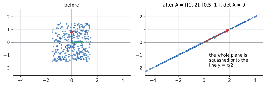
In that example the second column \((2, 1)\) is exactly twice the first column \((1, 0.5)\). Both basis vectors land on the same line, so their combinations (everything) land on that line. Singular means the columns are linearly dependent (Chapter 26): they fail to span the whole space.

Undoing \(A\) means: given an output \((p, q)\), find the input \((x, y)\) with

That’s a linear system, so solve it by elimination (Chapter 6). To eliminate \(y\), multiply the first equation by \(d\) and the second by \(b\), and subtract:

To eliminate \(x\), multiply the first by \(c\), the second by \(a\), and subtract the first from the second: \((ad - bc)\,y = aq - cp\). If \(ad - bc \neq 0\), divide:

The matrix taking \((p, q)\) back to \((x, y)\) is the inverse:

Swap the diagonal, negate the off-diagonal, divide by the determinant. And there’s the determinant, appearing on its own: if it’s zero, you’d divide by zero, which is the algebra’s way of saying "this can’t be undone".

Invert \(A = \begin{bmatrix} 3 & 1 \\ 5 & 2 \end{bmatrix}\) and use it to solve \(3x + y = 5\), \(5x + 2y = 9\). Try it: Check this inverse; Solve the system.

Check in the original equations: \(3 + 2 = 5\) ✓, \(5 + 4 = 9\) ✓.

Any system of linear equations can be written as one matrix equation. The system

Check by the row view: row 1 of \(A\) dotted with \(\mathbf{x}\) is \(2x + y - z\), the first left-hand side. This compact form is how systems are written in every linear-algebra paper and every numerical library.

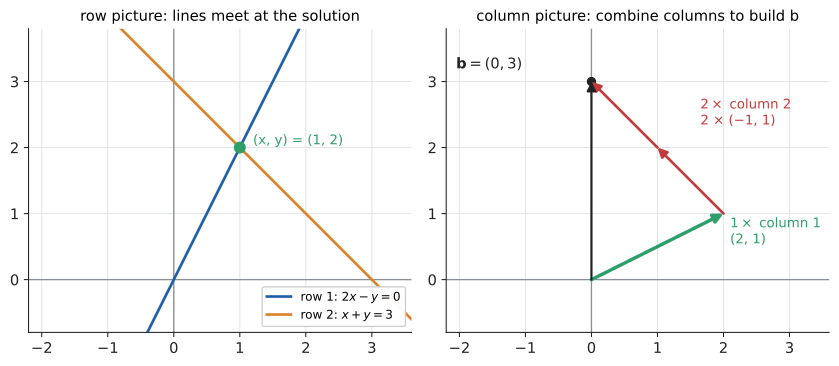
Chapter 6 taught you the row picture: each equation is a line (or plane), and the solution is where they all meet. Matrices add the column picture: \(A\mathbf{x}\) is a combination of the columns of \(A\), so solving \(A\mathbf{x} = \mathbf{b}\) asks

and, as a transformation: which input does \(A\) send to \(\mathbf{b}\)? That gives a clean geometric account of the three cases from Chapter 6:

The rank of a matrix is the dimension of its output: the number of independent directions the columns span. A \(3\times 3\) matrix of rank 3 fills all of space (invertible); rank 2 flattens space onto a plane; rank 1 crushes it onto a line; rank 0 is the zero matrix. The singular example above has rank 1. Rank is the honest measure of how much information a transformation preserves, and it returns in Chapter 28 as the key to compressing data with low-rank approximations.

The transpose \(A^\mathsf{T}\) of a matrix flips it across its main diagonal: rows become columns. If \(A\) is \(m\times n\), then \(A^\mathsf{T}\) is \(n\times m\), with \((A^\mathsf{T})_{ij} = a_{ji}\).

The transpose has less obvious geometry than the other operations, but it’s everywhere in practice, for three reasons.

1. It turns dot products into matrix products. Treat a column vector as an \(n\times 1\) matrix. Then \(\mathbf{a}^\mathsf{T}\) is \(1\times n\), and \(\mathbf{a}^\mathsf{T}\mathbf{b}\) is \((1\times n)(n\times 1) = 1\times 1\): a single number, which is exactly \(\mathbf{a}\cdot\mathbf{b}\). That’s why papers write \(\mathbf{q}^\mathsf{T}\mathbf{d}\) for the dot product, and \(\mathbf{x}^\mathsf{T}A\mathbf{x}\) for "transform \(\mathbf{x}\), then dot it with itself".

2. It reverses products: \((AB)^\mathsf{T} = B^\mathsf{T}A^\mathsf{T}\), the same socks-and-shoes reversal as the inverse.

3. For rotations, it is the inverse. The columns of a rotation matrix are perpendicular unit vectors (\(\mathbf{e}_1\) and \(\mathbf{e}_2\) rotated together). In \(R^\mathsf{T}R\), entry \((i, j)\) is (column \(i\)) \(\cdot\) (column \(j\)), which is 1 when \(i = j\) and 0 otherwise. So \(R^\mathsf{T}R = I\) and \(R^{-1} = R^\mathsf{T}\): inverting a rotation costs nothing. Matrices with orthonormal columns are called orthogonal matrices; they are the rigid motions (rotations and reflections) that preserve all lengths and angles.

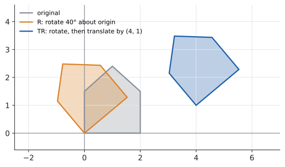
Rotating a sprite about its own centre, rather than about the origin, requires moving it to the origin, rotating, and moving it back. But moving (translation) isn’t linear: it doesn’t fix the origin, so no \(2\times 2\) matrix can do it. That spoils the plan of combining every transformation into one matrix.

Write the 2D point \((x, y)\) as the 3D vector \((x, y, 1)\). Now consider the \(3\times 3\) matrix

The constant 1 in the third slot, multiplied by the third column, smuggles in the shift. In three dimensions, translation is a shear that slides the plane \(z = 1\) sideways, and shears are linear. Rotations and scalings embed by putting their \(2\times 2\) matrix in the top-left corner with a 1 in the bottom-right. Now everything, including translation, is a matrix, and any sequence of moves collapses into one matrix by multiplication.

This also encodes the point/vector distinction from Chapter 26. A point gets a final coordinate 1 and is translated. A direction vector gets a final coordinate 0, so translation leaves it alone, which is correct: moving a spaceship doesn’t change which way "forward" is. Subtracting two points (1 − 1 = 0) gives a vector, automatically.

Rotate the points \((2, 1)\), \((3, 1)\), \((3, 2)\) by \(90^\circ\) about the point \((2, 1)\). Plan (read right to left): translate by \((-2, -1)\) so the pivot is at the origin, rotate, translate back. Try it: Rotate then translate the house; Rotate about a point.

By hand for \((3, 2)\): subtract the pivot, \((1, 1)\); rotate by \(90^\circ\), \((p, q) \mapsto (-q, p)\), giving \((-1, 1)\); add the pivot back, \((1, 2)\). In code, all three points at once, stored as columns:

The pivot \((2, 1)\) stays fixed, \((3, 1)\) swings up to \((2, 2)\), and \((3, 2)\) goes to \((1, 2)\), matching the hand calculation. (The np.round hides rounding noise like 6e-17 from \(\cos 90^\circ\) in floating point.)

A neural network takes a vector in (an image’s pixels, a sentence’s embedding) and produces a vector out (class probabilities, a next-word distribution). In between are layers. What does a layer actually compute?

A dense (fully connected) layer from \(n\) inputs to \(m\) outputs computes

where \(W\) is an \(m\times n\) weight matrix, \(\mathbf{b}\) an \(m\)-vector of biases, and \(\sigma\) a simple function applied to each entry separately, such as the ReLU \(\sigma(z) = \max(0, z)\). Read it with this chapter’s eyes:

Training adjusts the entries of \(W\) and \(\mathbf{b}\) using gradients (Chapter 20). But running a network, called inference, is almost entirely matrix multiplication.

Try it: Two linear layers collapse.

The last two lines show the trick that makes GPUs so effective: instead of 32 matrix–vector products, stack the inputs as rows of a matrix \(X\) and do one matrix–matrix product. Note the transpose: with inputs as rows, \(X W_1^\mathsf{T}\) has row \(i\) equal to \((W_1\mathbf{x}_i)^\mathsf{T}\). Mismatched shapes in exactly this spot are the most common bug in hand-written ML code; when NumPy complains, write the shapes of every factor down and check the inner dimensions.