Volume 2: Continuous Mathematics · Part VII: Linear Algebra
Chapter 26. Vectors
A number like 5 tells you how much. Plenty of quantities need more than that: a displacement of 5 km is useless unless you know which way, and a force of 5 newtons pushes in some direction. Vectors are the mathematics of "how much, and which way". This chapter rebuilds them from two complementary viewpoints: arrows you can draw, and lists of numbers you can compute with. We add and scale vectors, measure their length, and meet the single most useful operation in applied linear algebra, the dot product, which turns out to measure angle, projection, work done, brightness of a pixel, and the relevance of a document to a search query. We finish by stretching the humble \((3, 4)\) into the 768-dimensional embeddings that power modern semantic search, and by noting where three-dimensional intuition stops being trustworthy.
Why this chapter matters. Vectors are how both physics and software describe the world. A sat-nav adds displacement vectors, a game engine adds velocity vectors sixty times a second, a phone’s step counter measures the length of an acceleration vector, and every search box and recommendation feed ranks results by the angle between vectors. The handful of operations in this chapter (add, scale, measure, dot) is the vocabulary all of them share.
26.1. Quantities with direction
26.1.1. The problem
You leave a campsite and walk 3 km due east, then 4 km due north. How far are you from camp, and in which direction?
You already know how to answer this. Draw the two legs as a right angle, use Pythagoras for the straight-line distance, \(\sqrt{3^2 + 4^2} = 5\) km, and use trigonometry for the direction, \(\tan^{-1}(4/3) \approx 53.1^\circ\) north of east. But notice what you had to keep track of. Neither "3" nor "4" alone described a leg of the walk; each was a distance in a direction. And the answer, too, is a distance in a direction.
Physics is full of such quantities. If you took Mechanics at A-level, you spent a year with them: displacement, velocity, acceleration, force, momentum. All of them need a size and a direction. Two forces of 10 N acting on a box might cancel completely (opposite directions), add to 20 N (same direction), or combine to about 14.1 N (at right angles). The number 10 alone can’t tell you which.
So we need a mathematical object that carries direction as well as size, and rules for combining such objects that match what happens in the world. That object is the vector.
26.1.2. Intuition: an arrow, or a list of numbers
There are two ways to picture a vector, and the whole of linear algebra gets easier once you can switch between them without effort.
The arrow view. A vector is an arrow: it has a length and points in a direction. Crucially, it has no fixed position. The displacement "3 km east, 4 km north" is the same displacement whether you start at the campsite or at the car park. Slide the arrow anywhere without rotating or stretching it and it’s still the same vector.
The list view. Put the arrow’s tail at the origin of a coordinate system. Its tip lands at some point, say \((3, 4)\). Those two numbers record exactly how far the arrow goes in each axis direction, and they determine the arrow completely. So a vector is the list \((3, 4)\).
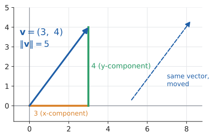
The arrow view gives you geometry: you can see addition, angles and projections. The list view gives you computation: you can add, multiply and store vectors in an array. The list view also generalises effortlessly. An arrow in 768 dimensions is impossible to draw, but a list of 768 numbers is just an array, and every rule in this chapter applies to it unchanged.
|
Scalar and vector
A scalar is an ordinary single number: a size with no direction (mass 4 kg, temperature 20 °C, speed 30 m/s). A vector is a quantity with both magnitude (size) and direction (displacement 30 m north-east, velocity 30 m/s due south). In the list view, a vector in \(n\) dimensions is an ordered list of \(n\) real numbers. The word "scalar" comes from the fact that multiplying a vector by a number scales it. |
|
Component
The components of a vector are the numbers in its list, one per axis. The vector \((3, 4)\) has x-component 3 and y-component 4. In general the \(i\)-th component of \(\mathbf{v}\) is written \(v_i\), so \(\mathbf{v} = (v_1, v_2, \ldots, v_n)\). The set of all lists of \(n\) real numbers is written \(\mathbb{R}^n\) ("R-n"), so \((3, 4) \in \mathbb{R}^2\) means "(3, 4) is a vector in two-dimensional real space". |
26.1.3. Vocabulary and notation
Vector notation varies between textbooks, countries and fields. You’ll meet all of these, and they mean the same thing.
|
Vector notation
In this book, vectors are bold. We write them as tuples in running text to save space and as columns inside calculations, especially once matrices arrive in Chapter 27. |
|
Points versus vectors
The point \((3, 4)\) and the vector \((3, 4)\) are written identically but are different kinds of thing. A point is a location; a vector is a displacement. The point \((3, 4)\) is "where the vector \((3, 4)\) lands if its tail is at the origin". The difference matters in practice: subtracting two points gives a vector (the displacement from one to the other), and adding a vector to a point gives a new point. Adding two points has no physical meaning: "London plus Paris" is not a place. Graphics programmers meet this distinction head-on, and it’s exactly what homogeneous coordinates in Chapter 27 encode. |
|
Why "vector"?
"Vector" is Latin for carrier, from vehere, to carry (the same root as "vehicle"). Astronomers used it for the imaginary line carrying a planet around the sun. The modern mathematical sense came from William Rowan Hamilton in the 1840s, as part of his quaternions (four-dimensional numbers he famously carved into Dublin’s Broom Bridge). Quaternions were clumsy for everyday physics, and in the 1880s Josiah Willard Gibbs in America and Oliver Heaviside in England independently stripped them down to the vector algebra used today: the dot product, the cross product, and the bold-letter notation. Biologists still use the older sense: a mosquito is a "vector" because it carries malaria. |
26.2. Adding and scaling vectors
26.2.1. The problem
A light aircraft points due north and flies at 200 km/h through the air. A wind blows from the west at 50 km/h, so the air itself is moving east. What is the plane’s actual velocity over the ground?
The plane’s motion is the result of two motions happening at once. Each is a vector, and we need a rule for combining them.
26.2.2. Intuition: tip to tail
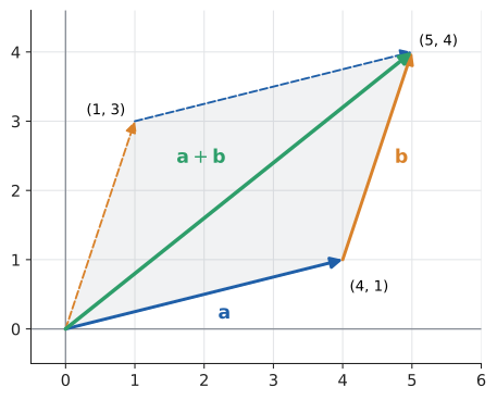
Think about displacements first, because they are the easiest to picture. If you walk along vector \(\mathbf{a}\), then along vector \(\mathbf{b}\), your total displacement is the single arrow from where you started to where you ended. Draw \(\mathbf{b}\) starting at the tip of \(\mathbf{a}\), then draw an arrow from the tail of \(\mathbf{a}\) to the tip of \(\mathbf{b}\). That arrow is \(\mathbf{a} + \mathbf{b}\). This is the tip-to-tail rule, also called the triangle law.
If you do the walks in the other order, \(\mathbf{b}\) first, you trace the other two sides of a parallelogram and end up in the same place. So \(\mathbf{a} + \mathbf{b} = \mathbf{b} + \mathbf{a}\), and the sum is the diagonal of the parallelogram the two vectors span. That’s the parallelogram law, and it’s how physicists add forces acting at a single point.
26.2.3. Why it works: components add independently
Look at the x-coordinates in the diagram. Walking along \(\mathbf{a}\) moves you 4 units right; then \(\mathbf{b}\) moves you 1 more. Total: 5. The y-coordinates are independent of this: 1 up, then 3 more, total 4. Horizontal and vertical motions don’t interfere with each other, so you add them separately:
That is the whole rule, in any number of dimensions: add component by component. The arrow picture and the list calculation always agree, which is why both views are legitimate.
26.2.4. Scaling: stretch, shrink, flip
Walking along \(\mathbf{v}\) twice is \(\mathbf{v} + \mathbf{v}\), which in components is every entry doubled. We write it \(2\mathbf{v}\). More generally, for any scalar \(c\), the scalar multiple \(c\mathbf{v}\) multiplies every component by \(c\):
Geometrically, \(c\mathbf{v}\) points along the same line as \(\mathbf{v}\) and is \(|c|\) times as long. If \(c > 1\) it stretches, if \(0 < c < 1\) it shrinks, and if \(c < 0\) it also flips to point the opposite way. \(0\mathbf{v}\) is the zero vector \(\mathbf{0} = (0, 0)\), the only vector with no direction.
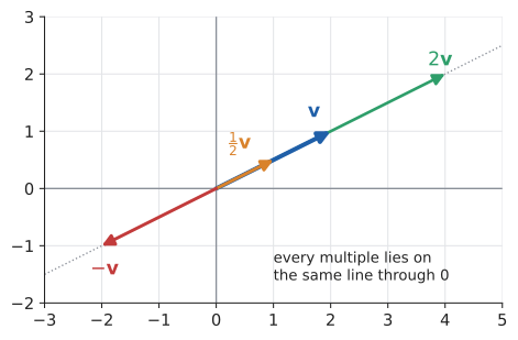
Subtraction follows: \(\mathbf{a} - \mathbf{b} = \mathbf{a} + (-1)\mathbf{b}\). Its geometric meaning is worth memorising: \(\mathbf{a} - \mathbf{b}\) is the arrow from the tip of \(\mathbf{b}\) to the tip of \(\mathbf{a}\). (Check: start at \(\mathbf{b}\), add \(\mathbf{a} - \mathbf{b}\), arrive at \(\mathbf{a}\).) This is why "the vector from point \(P\) to point \(Q\)" is \(Q - P\).
|
Vector arithmetic laws
For vectors \(\mathbf{a}, \mathbf{b}, \mathbf{c}\) in \(\mathbb{R}^n\) and scalars \(s, t\):
Each follows immediately from the matching law for ordinary numbers, applied one component at a time. Any collection of objects obeying these rules is called a vector space; that abstraction is why polynomials, audio signals and images can all be treated as vectors. |
Input: vectors \(\mathbf{a} = (a_1, \ldots, a_n)\), \(\mathbf{b} = (b_1, \ldots, b_n)\) of the same dimension; scalars \(s, t\).
Steps:
-
Check the dimensions match. If they don’t, the sum is undefined; stop.
-
Multiply every component of \(\mathbf{a}\) by \(s\) and every component of \(\mathbf{b}\) by \(t\).
-
Add the results position by position: the \(i\)-th component of the answer is \(s a_i + t b_i\).
Output: the vector \(s\mathbf{a} + t\mathbf{b} = (s a_1 + t b_1, \ldots, s a_n + t b_n)\).
26.2.5. Worked example: the aircraft in a crosswind
Set up axes with \(x\) pointing east and \(y\) pointing north, units km/h.
-
Air velocity (where the plane points): \(\mathbf{p} = (0, 200)\).
-
Wind velocity (blowing from the west means moving towards the east): \(\mathbf{w} = (50, 0)\).
Ground velocity is the sum:
To turn this back into "speed and direction", use Pythagoras and the tangent:
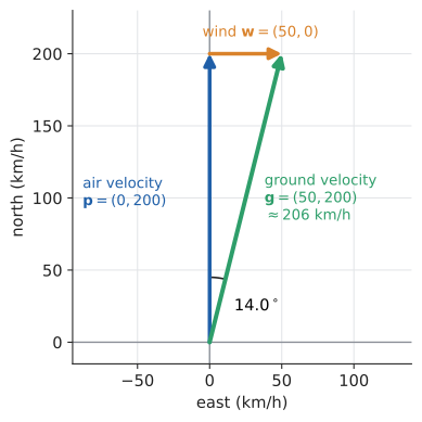
The plane travels slightly faster than its airspeed and drifts 14° off course. A pilot who wants to track due north must point slightly west so that the wind’s push cancels; finding that heading is a nice exercise below.
26.2.6. Worked example: three forces in equilibrium
A ring is held still by three ropes. Two of them pull with forces \(\mathbf{F}_1 = (3, 4)\) N and \(\mathbf{F}_2 = (-5, 2)\) N. What force must the third rope supply?
"Held still" (in equilibrium) means the forces sum to zero, Newton’s first law. So
The third rope pulls with \((2, -6)\) N, which has magnitude \(\sqrt{4 + 36} = \sqrt{40} \approx 6.32\) N, pointing right and steeply down. Drawn tip to tail, the three forces form a closed triangle: you end where you began.
26.2.7. Alternative approach: magnitude-and-angle form
Mechanics problems often give vectors as "a speed and a bearing" rather than as components. You can add those directly using the law of cosines on the triangle, but that’s error-prone and doesn’t scale beyond two vectors. The reliable method is: convert everything to components, add, convert back. A vector of length \(r\) at angle \(\theta\) above the positive x-axis has components
straight from the unit circle (Chapter 13). After adding, recover the length with Pythagoras and the angle with \(\tan^{-1}\) (or better, atan2, which gets the quadrant right). Choose components whenever more than two vectors are involved, or whenever you’ll compute.
|
Drag the arrows
Two draggable arrows \(\mathbf{a}\) and \(\mathbf{b}\) start at the origin. The app draws \(\mathbf{a} + \mathbf{b}\) both tip-to-tail and as the parallelogram diagonal, and shows the component arithmetic updating live. A slider for \(c\) shows \(c\mathbf{a}\) stretching, shrinking, and flipping as \(c\) passes through zero. Try it: Drag the arrows |
26.3. Exercises: adding and scaling
-
(Recognition) Which of these are vectors and which are scalars: temperature, wind velocity, mass, the force of gravity on a book, the price of a book?
-
(Application) With \(\mathbf{a} = (2, -1, 4)\) and \(\mathbf{b} = (0, 3, -2)\), compute \(3\mathbf{a} - 2\mathbf{b}\).
-
(Application) Points \(P = (1, 5)\) and \(Q = (4, 1)\). Find the vector \(\overrightarrow{PQ}\) and the midpoint of \(PQ\) using vectors.
-
(Problem solving) In the aircraft example, what heading should the pilot point (air velocity of magnitude 200 km/h) so that the ground track is due north? What’s the resulting ground speed?
Answers
-
Vectors: wind velocity, the force of gravity (it points down). Scalars: temperature, mass, price.
-
\(3\mathbf{a} = (6, -3, 12)\), \(2\mathbf{b} = (0, 6, -4)\). Subtract component by component: \((6 - 0,\ -3 - 6,\ 12 - (-4)) = (6, -9, 16)\).
-
\(\overrightarrow{PQ} = Q - P = (4 - 1, 1 - 5) = (3, -4)\). The midpoint is halfway along: \(P + \tfrac{1}{2}\overrightarrow{PQ} = (1, 5) + (1.5, -2) = (2.5, 3)\). (Equivalently \(\tfrac{1}{2}(P + Q)\).)
-
Let the air velocity be \(\mathbf{p} = (p_x, p_y)\) with \(p_x^2 + p_y^2 = 200^2\). Ground velocity \(\mathbf{p} + (50, 0)\) must have zero x-component, so \(p_x = -50\). Then \(p_y = \sqrt{40\,000 - 2500} = \sqrt{37\,500} \approx 193.6\). The pilot points \(\sin^{-1}(50/200) \approx 14.5^\circ\) west of north, and the ground speed is about \(193.6\) km/h, slower than the airspeed because part of the engine’s effort cancels the wind.
26.4. Length, distance, and unit vectors
26.4.1. The problem
A game character moves with velocity \((1, 0)\) when you press the right arrow and \((0, 1)\) when you press up. Press both, and the code adds them: \((1, 1)\). Players soon notice that moving diagonally is faster than moving straight. How much faster, and how do you fix it?
To answer, we need the length of a vector, and a way to keep a direction while setting the length to whatever we want.
26.4.2. Length from Pythagoras, in any dimension
In two dimensions, the arrow \((v_1, v_2)\) is the hypotenuse of a right triangle with legs \(|v_1|\) and \(|v_2|\), so its length is \(\sqrt{v_1^2 + v_2^2}\). For \((1, 1)\) that’s \(\sqrt{2} \approx 1.414\): diagonal movement is about 41% faster. That’s the bug.
In three dimensions, apply Pythagoras twice. The vector \((v_1, v_2, v_3)\) has a "shadow" \((v_1, v_2, 0)\) on the floor, of length \(\sqrt{v_1^2 + v_2^2}\). The full vector rises vertically \(v_3\) above the end of that shadow, making a second right triangle:
Nothing stops the pattern there. Each new axis is perpendicular to all the previous ones, so each adds one more squared term. In \(n\) dimensions, define the length the same way:
|
Magnitude (norm) and summation notation
The magnitude, length or norm of \(\mathbf{v}\) is written \(\|\mathbf{v}\|\) (double bars; some books use single bars \(|\mathbf{v}|\)). It’s the Euclidean norm, also called the L2 norm and written \(\|\mathbf{v}\|_2\) in machine-learning papers. The symbol \(\sum_{i=1}^{n} v_i^2\) is summation notation: \(\Sigma\) (capital Greek sigma, for "sum") means "add up", the index \(i\) runs from the value below (1) to the value above (\(n\)), and \(v_i^2\) is the term being added for each \(i\). So \(\sum_{i=1}^{3} v_i^2 = v_1^2 + v_2^2 + v_3^2\). In code it’s |
The distance between two points \(P\) and \(Q\) is the length of the vector between them, \(\|Q - P\|\). In two dimensions this is exactly the distance formula from Chapter 10; now it works in any dimension.
26.4.3. Unit vectors: direction without size
A unit vector has length 1. Dividing any nonzero vector by its own length produces a unit vector pointing the same way:
This is called normalising \(\mathbf{v}\). The hat notation \(\hat{\mathbf{v}}\) ("v-hat") is the usual marker for a unit vector. Normalising throws away the magnitude and keeps the pure direction; you can then multiply by any length you like. The special unit vectors along the axes, \(\mathbf{i} = (1, 0, 0)\), \(\mathbf{j} = (0, 1, 0)\), \(\mathbf{k} = (0, 0, 1)\), are the standard basis vectors, also written \(\mathbf{e}_1, \mathbf{e}_2, \mathbf{e}_3\).
Input: a vector \(\mathbf{v}\).
Steps:
-
Compute \(\|\mathbf{v}\| = \sqrt{\sum v_i^2}\).
-
If \(\|\mathbf{v}\| = 0\) (or is tiny compared with the precision of your data), stop: the zero vector has no direction. Report an error or return a sensible default.
-
Divide every component by \(\|\mathbf{v}\|\).
Output: the unit vector \(\hat{\mathbf{v}}\). Check: its length should be 1 (up to rounding).
26.4.4. Worked example
Normalise \(\mathbf{v} = (2, -1, 2)\). Try it: Normalise (2, −1, 2).
And the game fix: before applying movement, normalise the input direction (when it isn’t zero) and multiply by the desired speed \(s\). Diagonal input \((1, 1)\) becomes \(s \cdot (0.707, 0.707)\), whose length is \(s\), the same as straight movement.
26.4.5. Where you’d use this
-
Everyday: your phone’s step counter. The accelerometer reports a 3D vector in m/s², but you might hold the phone in any orientation, so the individual components are meaningless on their own. The step counter uses the length. Standing still, a reading like \((3, 6, 7)\) has length \(\sqrt{9 + 36 + 49} = \sqrt{94} \approx 9.7\), which is just gravity. Mid-stride, \((6, 12, 4)\) has length \(\sqrt{36 + 144 + 16} = \sqrt{196} = 14\). Count the peaks of the length and you’ve counted steps, whichever pocket the phone is in.
-
Science and engineering: a drone’s speed from its velocity components, the resultant of several forces, and the distance between two atoms in a molecule (from their 3D coordinates) are all \(\|\mathbf{v}\|\) or \(\|Q - P\|\). Surveyors and GPS receivers compute 3D distances to satellites exactly this way.
-
Computing: colour difference. Two pixels \((255, 100, 50)\) and \((250, 110, 40)\) in RGB differ by \((5, -10, 10)\), a distance of \(\sqrt{25 + 100 + 100} = 15\); image editors use this (or a perceptual variant) for "magic wand" selection. The same distance, in more dimensions, drives k-nearest-neighbour classifiers and recommendation lookups. And unit vectors are everywhere in graphics: surface normals, camera directions and light directions are all normalised before use, as the Lambert shading sidebar below shows.
|
The zero vector cannot be normalised
\(\mathbf{0}/\|\mathbf{0}\|\) is \(0/0\). In code this produces |
26.5. Linear combinations and span
26.5.1. The problem
You have two moves available: \(\mathbf{a} = (2, 1)\) and \(\mathbf{b} = (1, -1)\), and you may use each any real number of times (including fractions and negatives). Can you reach the point \((7, 1)\)? Can you reach every point?
26.5.2. Intuition
An expression like \(x\mathbf{a} + y\mathbf{b}\), scaled vectors added together, is called a linear combination of \(\mathbf{a}\) and \(\mathbf{b}\). Think of \(\mathbf{a}\) and \(\mathbf{b}\) as two directions on a strange compass, and \(x\), \(y\) as how far you travel along each. The span of \(\mathbf{a}\) and \(\mathbf{b}\) is the set of everywhere you can reach.
-
One nonzero vector spans a line through the origin (all its multiples, as in the scalar-multiple diagram).
-
Two vectors that point in genuinely different directions span a plane. In \(\mathbb{R}^2\), that plane is everything.
-
Two vectors that lie on the same line (one is a multiple of the other) span only that line. The second adds nothing new.
-
Three vectors in \(\mathbb{R}^3\) span all of space, unless one of them lies in the plane of the other two.
26.5.3. Worked example: reaching \((7, 1)\)
We need \(x(2, 1) + y(1, -1) = (7, 1)\). Comparing components gives a system of equations (Chapter 6): Try it: Reach (7, 1).
Adding the equations eliminates \(y\): \(3x = 8\), so \(x = 8/3\). Then \(y = x - 1 = 5/3\). Check: \(\tfrac{8}{3}(2, 1) + \tfrac{5}{3}(1, -1) = (\tfrac{16}{3} + \tfrac{5}{3},\ \tfrac{8}{3} - \tfrac{5}{3}) = (7, 1)\). ✓
The same elimination works for any target \((p, q)\): \(x = (p + q)/3\), \(y = (p - 2q)/3\). So \(\mathbf{a}\) and \(\mathbf{b}\) span the whole plane.
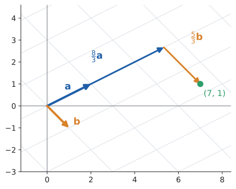
Notice the deep fact hiding here: asking whether a vector is a linear combination of others is the same as solving a system of linear equations. That equivalence is the beating heart of linear algebra, and Chapter 27 builds on it.
|
Linear combination, span, independence, basis
|
|
Two vectors in 3D are not "enough"
Counting vectors is not the same as counting directions. Two vectors in \(\mathbb{R}^3\) span at most a plane, never all of space. And \((1, 2, 3)\), \((2, 4, 6)\) and \((0, 1, 0)\) are three vectors but span only a plane, because the second is twice the first. When a feature vector in machine learning has 100 entries but they’re all computed from 5 underlying measurements, the data really lives in (at most) a 5-dimensional subspace. Spotting that hidden low dimension is exactly what PCA does in Chapter 28. |
26.5.4. Where you’d use this
-
Everyday: hitting a nutrition target. Per 100 g, cooked lentils give about 9 g protein and 20 g carbohydrate, and cooked rice about 3 g protein and 28 g carbohydrate. Each food is a vector, (protein, carbs) = \((9, 20)\) and \((3, 28)\). To hit 27 g protein and 124 g carbohydrate you need \(x(9, 20) + y(3, 28) = (27, 124)\), that is \(9x + 3y = 27\) and \(20x + 28y = 124\). The first gives \(y = 9 - 3x\); substituting, \(20x + 252 - 84x = 124\), so \(x = 2\) and \(y = 3\): 200 g of lentils and 300 g of rice. Diet-planning apps and animal-feed formulators solve exactly this, with dozens of nutrients.
-
Science: balancing a chemical equation. Record each molecule as a vector of atom counts (C, H, O): \(\text{CH}_4 = (1, 4, 0)\), \(\text{O}_2 = (0, 0, 2)\), \(\text{CO}_2 = (1, 0, 2)\), \(\text{H}_2\text{O} = (0, 2, 1)\). Balancing means finding coefficients with \(1(1, 4, 0) + 2(0, 0, 2) = (1, 4, 4) = 1(1, 0, 2) + 2(0, 2, 1)\), which is \(\text{CH}_4 + 2\text{O}_2 \to \text{CO}_2 + 2\text{H}_2\text{O}\): a linear combination problem.
-
Computing: every pixel colour is a linear combination \(r\,\mathbf{red} + g\,\mathbf{green} + b\,\mathbf{blue}\) of three basis colours. JPEG goes further: each 8×8 block of an image is rewritten as a linear combination of 64 fixed "cosine pattern" basis images, and compression keeps only the coefficients that matter. Animation tweens and gradients use the combination \((1 - t)\mathbf{a} + t\mathbf{b}\) ("lerp") to slide smoothly from \(\mathbf{a}\) at \(t = 0\) to \(\mathbf{b}\) at \(t = 1\).
|
Combination sliders
Fix two vectors \(\mathbf{a}\) and \(\mathbf{b}\). Two sliders control \(x\) and \(y\), and the app draws \(x\mathbf{a} + y\mathbf{b}\) with a faint trail. Sweep the sliders and watch the trail fill the plane. Then drag \(\mathbf{b}\) onto the line of \(\mathbf{a}\) and watch the reachable set collapse to a line. A "target" mode places a random point and asks the learner to find the coefficients. |
26.6. The dot product
26.6.1. The problem
Two very different questions turn out to have the same answer.
A Mechanics question. You drag a sled 5 m across flat snow, pulling on a rope with a 10 N force angled 60° above the horizontal. How much work do you do? Work is "force times distance moved in the direction of the force", so only part of your pull counts.
A data question. Two documents, or two users, or two songs, are represented by vectors of numbers. How similar are they? We’d like a single number that’s large when the vectors point the same way and small or negative when they don’t.
Both questions ask: how much do two vectors agree in direction, weighted by their sizes? The tool that answers it is the dot product.
26.6.2. The algebraic definition
Multiply matching components and add up:
The result is a scalar, not a vector, which is why it’s also called the scalar product (or inner product). For example,
The second calculation shows an important link: a vector dotted with itself is its length squared, \(\mathbf{v} \cdot \mathbf{v} = \|\mathbf{v}\|^2\). Directly from the definition, the dot product also satisfies
-
\(\mathbf{a} \cdot \mathbf{b} = \mathbf{b} \cdot \mathbf{a}\) (symmetric),
-
\(\mathbf{a} \cdot (\mathbf{b} + \mathbf{c}) = \mathbf{a} \cdot \mathbf{b} + \mathbf{a} \cdot \mathbf{c}\) (distributes over addition),
-
\((s\mathbf{a}) \cdot \mathbf{b} = s(\mathbf{a} \cdot \mathbf{b})\) (scalars pull out).
Each holds because it holds for every term \(a_i b_i\) separately.
That’s the mechanical definition. On its own it looks arbitrary: why multiply matching components? The answer is that this mechanical recipe secretly measures an angle.
26.6.3. Why it works: the geometric meaning
|
Law of cosines
In any triangle with sides \(a\), \(b\), \(c\), where \(\theta\) is the angle between sides \(a\) and \(b\) (opposite side \(c\)):
\[c^2 = a^2 + b^2 - 2ab\cos\theta.\]
When \(\theta = 90^\circ\), \(\cos\theta = 0\) and it reduces to Pythagoras. The \(-2ab\cos\theta\) term is the correction for the triangle not being right-angled. (Derived in Chapter 13.) |
Put the tails of \(\mathbf{a}\) and \(\mathbf{b}\) together, with angle \(\theta\) between them. The third side of the triangle runs from the tip of \(\mathbf{b}\) to the tip of \(\mathbf{a}\), which is the vector \(\mathbf{a} - \mathbf{b}\).
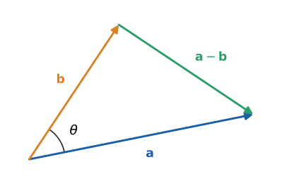
Now compute the squared length of the third side in two ways.
Using the dot product algebra:
Using the law of cosines with side lengths \(\|\mathbf{a}\|\), \(\|\mathbf{b}\|\), \(\|\mathbf{a} - \mathbf{b}\|\):
The left sides are equal, so the right sides are equal. Cancel \(\|\mathbf{a}\|^2 + \|\mathbf{b}\|^2\) from both and divide by \(-2\):
This is the central fact of the chapter. The "multiply and add" recipe, which a computer does in nanoseconds, equals "length times length times the cosine of the angle between", which is geometry. Two representations, one number.
|
Dot product
The dot product (scalar product, inner product) of two vectors of the same dimension is
\[\mathbf{a}\cdot\mathbf{b} = \sum_{i=1}^n a_i b_i = \|\mathbf{a}\|\,\|\mathbf{b}\|\cos\theta.\]
It is a scalar. Other notations: \(\langle \mathbf{a}, \mathbf{b} \rangle\) (mathematics, physics), \(\mathbf{a}^\mathsf{T}\mathbf{b}\) (linear algebra, "a-transpose b"; see Chapter 27), and |
26.6.4. What the sign tells you
Since lengths are positive, the sign of \(\mathbf{a}\cdot\mathbf{b}\) is the sign of \(\cos\theta\):
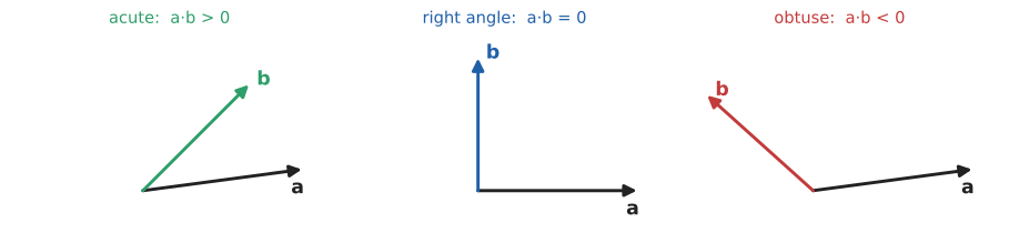
The middle case gets its own word. Vectors with \(\mathbf{a}\cdot\mathbf{b} = 0\) are orthogonal (perpendicular, at right angles). Earlier we found \((3, 4)\cdot(4, -3) = 0\): those two arrows are perpendicular, which you can confirm by sketching them. This is an astonishingly cheap perpendicularity test: no angles, no trigonometry, just multiply and add. In 768 dimensions, where you can’t sketch anything, it’s the only practical test.
|
Orthogonal
Two vectors are orthogonal if their dot product is zero. For nonzero vectors this means they meet at 90°. (The zero vector is orthogonal to everything, by this definition.) "Orthogonal" is the general-dimension word; "perpendicular" is usual in 2D and 3D geometry; "normal" is used for a vector perpendicular to a surface. A set of vectors that are mutually orthogonal and all of length 1 is orthonormal; the standard basis is the classic example. |
Input: nonzero vectors \(\mathbf{a}\), \(\mathbf{b}\) of the same dimension.
Steps:
-
Compute \(\mathbf{a}\cdot\mathbf{b} = \sum a_i b_i\).
-
Compute \(\|\mathbf{a}\|\) and \(\|\mathbf{b}\|\).
-
Compute \(\cos\theta = \dfrac{\mathbf{a}\cdot\mathbf{b}}{\|\mathbf{a}\|\,\|\mathbf{b}\|}\). (In code, clamp the result into \(\lbrack -1, 1]\) before the next step; rounding can push it to 1.0000000002.)
-
\(\theta = \cos^{-1}(\cos\theta)\), which lies between \(0^\circ\) and \(180^\circ\).
Output: the angle \(\theta\). If only "same way / perpendicular / opposite" matters, stop after step 1 and read the sign.
26.6.5. Worked example: angle between two 3D vectors
Find the angle between \(\mathbf{a} = (1, 2, 2)\) and \(\mathbf{b} = (2, -1, 2)\). Try it: Angle between two 3D vectors.
26.6.6. Worked example: work done dragging a sled
Work done by a constant force \(\mathbf{F}\) over a displacement \(\mathbf{d}\) is \(W = \mathbf{F}\cdot\mathbf{d}\). With the rope at 60°:
Check with the geometric form: \(\|\mathbf{F}\|\,\|\mathbf{d}\|\cos 60^\circ = 10 \cdot 5 \cdot 0.5 = 25\) J. The vertical part of your pull (8.66 N) does no work because the sled doesn’t move vertically: its dot product with the displacement is zero. That’s the physical meaning of orthogonality, and it’s why carrying a heavy bag across a level room does, by the physicist’s definition, no work on the bag.
26.6.7. Where you’d use this
-
Everyday: a shopping bill is a dot product. Quantities \(\mathbf{q} = (3, 2, 1)\) (pints of milk, loaves, jars of coffee) and prices \(\mathbf{p} = (1.20, 1.50, 4.00)\) give the total \(\mathbf{q}\cdot\mathbf{p} = 3.60 + 3.00 + 4.00 = 10.60\). Any weighted total is a dot product: a course grade from weighted assignments, a nutrition label’s calories from grams of fat, carbohydrate and protein, a portfolio’s value from holdings and share prices.
-
Science and engineering: work \(\mathbf{F}\cdot\mathbf{d}\) (above) and power \(\mathbf{F}\cdot\mathbf{v}\). A solar panel’s output follows Lambert’s cosine law: a 1.6 m² panel in 1000 W/m² sunshine collects 1600 W of sunlight when it faces the sun squarely, but only \(1600\cos 60^\circ = 800\) W when the sun is 60° away from its normal. That’s why solar farms use trackers that tilt the panels to follow the sun.
-
Computing: a single artificial neuron computes \(\mathbf{w}\cdot\mathbf{x} + b\) (Chapter 27), lighting uses \(\mathbf{n}\cdot\mathbf{l}\) (below), and testing \(\mathbf{a}\cdot\mathbf{b} = 0\) is the cheapest possible check for "perpendicular", used in collision detection and geometry code everywhere.
|
acos and floating point
|
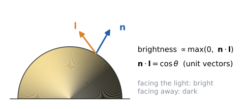
Why does the side of a ball facing a lamp look bright and the far side dark? A patch of matte surface receives light in proportion to how squarely it faces the light source. If \(\mathbf{n}\) is the unit surface normal (pointing straight out of the surface) and \(\mathbf{l}\) is the unit vector towards the light, the brightness is
where \(k_d\) is the surface’s colour (its diffuse reflectance). Face the light head-on: \(\mathbf{n}\cdot\mathbf{l} = 1\), full brightness. Tilt by 60°: \(\cos 60^\circ = 0.5\), half brightness. Face away: the dot product goes negative and the \(\max\) clamps it to zero, shadow. This is Lambert’s cosine law (1760), and one line of it, max(0.0, dot(n, l)), runs billions of times per second in every GPU’s fragment shaders.
26.7. Projections
26.7.1. The problem
A 4 kg box rests on a ramp inclined at 30°. Gravity pulls straight down. How much of that pull acts along the ramp (trying to slide the box) and how much acts into the ramp (pressing it against the surface)?
Equivalently: given a vector \(\mathbf{a}\) and a direction \(\mathbf{b}\), split \(\mathbf{a}\) into a part along \(\mathbf{b}\) and a part perpendicular to \(\mathbf{b}\). Mechanics calls this resolving a force. Linear algebra calls the first part the projection of \(\mathbf{a}\) onto \(\mathbf{b}\).
26.7.2. Intuition: the shadow
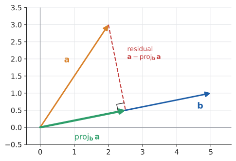
Shine a light perpendicular to the line of \(\mathbf{b}\). The shadow that \(\mathbf{a}\) casts on that line is its projection. What’s left over, from the tip of the shadow up to the tip of \(\mathbf{a}\), is perpendicular to \(\mathbf{b}\).
26.7.3. Why it works: deriving the formula
Let \(\hat{\mathbf{b}} = \mathbf{b}/\|\mathbf{b}\|\) be the unit vector along \(\mathbf{b}\). In the right triangle formed by \(\mathbf{a}\), its shadow and the residual, \(\mathbf{a}\) is the hypotenuse and the shadow is the side adjacent to angle \(\theta\). So the shadow’s (signed) length is
That number is the scalar projection (or component of \(\mathbf{a}\) along \(\mathbf{b}\)). It’s negative if \(\mathbf{a}\) points partly backwards. To get the projection as a vector, multiply this length by the unit direction:
The second form avoids square roots, which is handy by hand and in code. The perpendicular part is whatever’s left: \(\mathbf{a} - \operatorname{proj}_{\mathbf{b}}\mathbf{a}\).
|
Projection
A key reading: dotting with a unit vector measures the component in that direction. That’s why \(\mathbf{v}\cdot\mathbf{i}\) is just \(v_1\). |
Input: a vector \(\mathbf{a}\) and a nonzero direction vector \(\mathbf{b}\).
Steps:
-
Compute \(\mathbf{a}\cdot\mathbf{b}\) and \(\mathbf{b}\cdot\mathbf{b}\).
-
Compute the coefficient \(k = (\mathbf{a}\cdot\mathbf{b})/(\mathbf{b}\cdot\mathbf{b})\).
-
Parallel part: \(\mathbf{p} = k\,\mathbf{b}\).
-
Perpendicular part: \(\mathbf{r} = \mathbf{a} - \mathbf{p}\).
-
Check: \(\mathbf{r}\cdot\mathbf{b}\) should be 0 (up to rounding).
Output: \(\mathbf{p}\) (along \(\mathbf{b}\)) and \(\mathbf{r}\) (perpendicular), with \(\mathbf{a} = \mathbf{p} + \mathbf{r}\).
26.7.4. Worked example: the diagram’s numbers
Project \(\mathbf{a} = (2, 3)\) onto \(\mathbf{b} = (5, 1)\). Try it: Project a onto b.
In NumPy, where @ between two 1-D arrays is the dot product:
import numpy as np

a = np.array([2.0, 3.0])
b = np.array([5.0, 1.0])

def project(a, b):
    """Vector projection of a onto b."""
    return (a @ b) / (b @ b) * b

p = project(a, b)
r = a - p
print(p)            # the shadow of a on b's line
print(r)            # what's left over
print(r @ b)        # residual is perpendicular to b
[2.5 0.5] [-0.5 2.5] 0.0
26.7.5. Worked example: the box on the ramp
Take \(x\) horizontal and \(y\) vertical. The weight is \(\mathbf{W} = (0, -4 \times 9.8) = (0, -39.2)\) N. A unit vector pointing up the 30° ramp is \(\hat{\mathbf{u}} = (\cos 30^\circ, \sin 30^\circ) \approx (0.866, 0.5)\), and a unit vector perpendicular to the ramp, pointing out of its surface, is \(\hat{\mathbf{n}} = (-\sin 30^\circ, \cos 30^\circ) \approx (-0.5, 0.866)\). (Check: \(\hat{\mathbf{u}}\cdot\hat{\mathbf{n}} = -0.433 + 0.433 = 0\).)
These are the familiar Mechanics results \(mg\sin\theta\) and \(mg\cos\theta\), now obtained without drawing a single similar triangle. The ramp pushes back with a normal reaction of 33.9 N; friction must supply up to 19.6 N to stop the box sliding.
26.7.6. Choosing a method
For resolving forces in a 2D Mechanics problem, the trigonometric shortcuts (\(mg\sin\theta\), \(mg\cos\theta\)) are fastest if you draw the diagram correctly. The dot-product method is mechanical and immune to "was it sine or cosine?" errors, works in 3D and beyond, and is what you’d write in code. Use trig for quick sketches; use projection for anything you’ll compute or anything not in a plane.
26.7.7. Where you’d use this
-
Everyday and aviation: headwind and crosswind. A pilot landing on a runway, or a cyclist on a straight road, cares about two pieces of the wind: the part along the direction of travel and the part across it. A 30-knot wind blowing at 40° to the runway has a headwind component \(30\cos 40^\circ \approx 23.0\) knots and a crosswind component \(30\sin 40^\circ \approx 19.3\) knots. That second number decides whether a small aircraft may land (many have a crosswind limit around 15–20 knots).
-
Science: resolving forces on slopes, cables and bridges (as above); in surveying, splitting a measured displacement into its horizontal and vertical parts.
-
Computing: in a game, when a character runs into a wall you remove the into-the-wall part of its velocity and keep the projection along the wall, so it slides instead of stopping dead. Fitting a straight line to data by least squares (Chapter 31) is a projection too: the fitted values are the shadow of the data vector on the space of possible straight-line predictions, and the residuals are perpendicular to it.
|
Resolve a force
Drag a vector \(\mathbf{a}\) and a direction \(\mathbf{b}\). The app shows the shadow of \(\mathbf{a}\) on the line of \(\mathbf{b}\), the perpendicular residual with its right-angle marker, and the numbers \(\mathbf{a}\cdot\mathbf{b}\), \(k\) and \(\theta\). Rotate \(\mathbf{a}\) past 90° and watch the projection flip to point backwards as the dot product goes negative. A "ramp" mode tilts a slope and resolves the box’s weight live. Try it: Resolve a force |
26.8. Exercises: magnitude, dot product, projection
-
(Recognition) Without computing an angle, say whether the angle between \((3, -1)\) and \((1, 2)\) is acute, right, or obtuse.
-
(Application) Find a unit vector in the direction of \((4, -4, 2)\).
-
(Application) Find the angle between \((3, -1)\) and \((1, 2)\) to the nearest degree.
-
(Application) Decompose \(\mathbf{a} = (4, 2)\) into parts parallel and perpendicular to \(\mathbf{b} = (1, 1)\).
-
(Problem solving) Find all vectors \((x, y)\) orthogonal to \((2, 5)\), and give the one of length 1 with positive x-component.
-
(Problem solving) Show that for any vectors, \(\|\mathbf{a} + \mathbf{b}\|^2 = \|\mathbf{a}\|^2 + \|\mathbf{b}\|^2\) exactly when \(\mathbf{a}\cdot\mathbf{b} = 0\). What famous theorem is this?
Answers
-
\((3)(1) + (-1)(2) = 1 > 0\), so the angle is acute (but only just).
-
\(\|(4, -4, 2)\| = \sqrt{16 + 16 + 4} = \sqrt{36} = 6\). Unit vector: \((4, -4, 2)/6 = (\tfrac{2}{3}, -\tfrac{2}{3}, \tfrac{1}{3})\).
-
Dot product 1; lengths \(\sqrt{10}\) and \(\sqrt{5}\); \(\cos\theta = 1/\sqrt{50} \approx 0.1414\); \(\theta \approx 81.9^\circ \approx 82^\circ\).
-
\(\mathbf{a}\cdot\mathbf{b} = 6\), \(\mathbf{b}\cdot\mathbf{b} = 2\), \(k = 3\). Parallel: \((3, 3)\). Perpendicular: \((4, 2) - (3, 3) = (1, -1)\). Check: \((1, -1)\cdot(1, 1) = 0\). ✓
-
\(2x + 5y = 0\), so \(y = -\tfrac{2}{5}x\): all multiples of \((5, -2)\) (a line through the origin). Length \(\sqrt{29}\), so the unit vector is \((5, -2)/\sqrt{29} \approx (0.928, -0.371)\). (Handy trick: in 2D, \((a, b)\) is always perpendicular to \((b, -a)\) and \((-b, a)\).)
-
Expand: \(\|\mathbf{a} + \mathbf{b}\|^2 = (\mathbf{a} + \mathbf{b})\cdot(\mathbf{a} + \mathbf{b}) = \|\mathbf{a}\|^2 + 2\,\mathbf{a}\cdot\mathbf{b} + \|\mathbf{b}\|^2\). This equals \(\|\mathbf{a}\|^2 + \|\mathbf{b}\|^2\) exactly when \(2\,\mathbf{a}\cdot\mathbf{b} = 0\). It’s Pythagoras’s theorem (and its converse), valid in any number of dimensions.
26.9. Cosine similarity, embeddings, and search
26.9.1. The problem
A search engine holds a million documents. A user types a query. Which documents are most relevant?
This is the founding problem of information retrieval, and since the 1960s the dominant answer has been geometric: turn every document and every query into a vector, and rank documents by how closely their vectors point the same way as the query’s.
26.9.2. Documents as vectors
The simplest representation is a bag of words. Fix a vocabulary of \(n\) words. A document becomes a vector in \(\mathbb{R}^n\) whose \(i\)-th component counts how often word \(i\) appears. With only two vocabulary words, "matrix" and "graph", we can draw it:
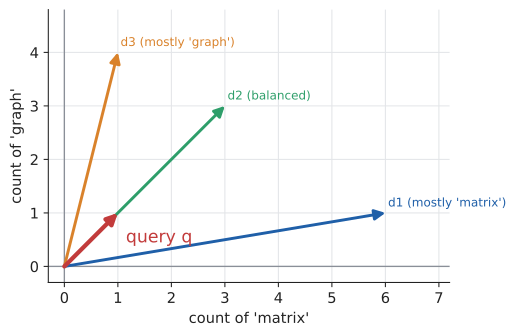
Should we rank by the raw dot product \(\mathbf{q}\cdot\mathbf{d}\)? It rewards documents that share words with the query, which is good. But \(\mathbf{q}\cdot\mathbf{d} = \|\mathbf{q}\|\,\|\mathbf{d}\|\cos\theta\) also grows with \(\|\mathbf{d}\|\), so a long document beats a short one just by being long. Paste a document into itself ten times and its score goes up tenfold, without becoming any more relevant.
The fix is to divide out the lengths, leaving only the angle. That’s cosine similarity:
It lies between \(-1\) and \(1\) (between 0 and 1 for count vectors, which have no negative entries), and depends only on direction.
26.9.3. Worked example: length bias
Query \(\mathbf{q} = (1, 1)\) (the words "matrix graph"). Three documents: \(A = (10, 10)\), a long document using both words equally; \(B = (2, 0)\), a short one about matrices only; \(C = (1, 1)\), a short one using both. Try it: Dot product versus cosine.
The raw dot product says \(A\) is ten times as relevant as \(C\); cosine similarity correctly says they’re equally on-topic, and both beat \(B\), which covers only half the query.
26.9.4. TF-IDF: weighting the components
Raw counts have another flaw: "the" appears everywhere and dominates every vector while telling you nothing. TF-IDF reweights each component by how informative the word is. A word’s document frequency \(\text{df}(w)\) is the number of documents containing it; out of \(N\) documents its inverse document frequency is \(\text{idf}(w) = \log(N / \text{df}(w))\), which is zero for a word in every document and large for a rare one. Each component becomes term frequency times IDF. Everything else, including cosine ranking, stays the same. Try it: Rank with TF-IDF.
import math
from collections import Counter

corpus = [
    "the matrix rotates the vector",
    "the graph has a vertex and an edge",
    "a vector is an arrow and a vector is a list",
]
tokenised = [doc.split() for doc in corpus]
vocab = sorted({w for doc in tokenised for w in doc})
N = len(corpus)
df = Counter(w for doc in tokenised for w in set(doc))      # document frequency
idf = {w: math.log(N / df[w]) for w in vocab}

def tfidf(tokens):
    tf = Counter(tokens)
    return [tf[w] * idf[w] for w in vocab]

vectors = [tfidf(doc) for doc in tokenised]
query = tfidf("vector arrow".split())

def cosine(a, b):
    num = sum(x * y for x, y in zip(a, b))
    den = math.sqrt(sum(x * x for x in a)) * math.sqrt(sum(y * y for y in b))
    return num / den if den else 0.0

for doc, vec in zip(corpus, vectors):
    print(f"{cosine(query, vec):.3f}  {doc}")
0.078 the matrix rotates the vector 0.000 the graph has a vertex and an edge 0.421 a vector is an arrow and a vector is a list
The third document wins: it contains both query words, and "arrow" is rare (high IDF). The first scores a little for "vector". The second shares no query words and scores zero, its vector orthogonal to the query’s.
|
TF-IDF and cosine similarity
|
26.9.5. From \((3, 4)\) to 768 dimensions: embeddings
Bag-of-words vectors have a blind spot. "Car" and "automobile" are different vocabulary entries, so the corresponding axes are orthogonal, and a query for one scores zero against a document using only the other. The vectors capture spelling, not meaning.
Modern systems use embeddings: vectors produced by a trained neural network, designed so that texts with similar meanings get vectors pointing in similar directions. A typical sentence embedding has 384, 768, 1024 or more components. Here is the important point, and it’s worth slowing down for: mathematically, an embedding is exactly the same kind of object as \((3, 4)\). It’s a list of real numbers. Its length is \(\sqrt{\sum v_i^2}\), with 768 terms instead of 2. Its dot product with another embedding is \(\sum a_i b_i\), with 768 products instead of 2. The angle between two embeddings is \(\cos^{-1}\) of the normalised dot product, defined by the very formula we derived from the law of cosines. Nothing in our derivation used the fact that we were in two dimensions; we only used the algebraic rules of the dot product. You can’t draw a 768-dimensional arrow, but every calculation you’d do on the drawing still works.
What’s different is what the components mean. In \((3, 4)\) the components are "east" and "north". In an embedding, no single component has a clean meaning; meaning lives in directions, combinations of many components. Similar meanings point similar ways; that’s all the geometry needs.
26.9.6. Reading \(\mathbf{q}\cdot\mathbf{d}\)
You’ll meet the expression \(\mathbf{q}\cdot\mathbf{d}\) constantly in information-retrieval and machine-learning papers. You can now unpack it completely:
-
\(\mathbf{q}\) is the query’s vector and \(\mathbf{d}\) a document’s vector, in the same space (same dimension, same meaning of each axis).
-
\(\mathbf{q}\cdot\mathbf{d} = \sum_i q_i d_i\) is computed by multiplying matching components and adding: \(n\) multiplications and \(n - 1\) additions.
-
Geometrically it’s \(\|\mathbf{q}\|\,\|\mathbf{d}\|\cos\theta\): large when the vectors are long and aligned.
-
Embedding systems usually normalise every vector to length 1 when they’re stored. Then \(\mathbf{q}\cdot\mathbf{d} = \cos\theta\) exactly: the dot product is cosine similarity, without the divisions. That’s why papers often write the dot product and mean the cosine.
-
For unit vectors, Euclidean distance carries the same information too:
\[\|\mathbf{q} - \mathbf{d}\|^2 = \|\mathbf{q}\|^2 + \|\mathbf{d}\|^2 - 2\,\mathbf{q}\cdot\mathbf{d} = 2 - 2\cos\theta,\]so ranking by largest cosine, largest dot product, or smallest distance gives the same order. Which "metric" a vector database asks you to pick matters only for unnormalised vectors.
26.9.7. Worked example: semantic search in NumPy
Here are five toy documents with 4-dimensional "embeddings" (real ones come from a model, but the search step is identical). Storing the documents as the rows of a 2-D array lets NumPy compute all five dot products in one operation.
import numpy as np

# Five toy "documents", each already embedded as a 4-dimensional vector.
docs = ["cat care guide", "kitten adoption", "stock market news",
        "interest rates rise", "dog training tips"]
D = np.array([
    [0.9, 0.1, 0.0, 0.3],
    [0.8, 0.2, 0.1, 0.1],
    [0.0, 0.9, 0.4, 0.0],
    [0.1, 0.8, 0.6, 0.0],
    [0.6, 0.0, 0.1, 0.8],
])
q = np.array([0.85, 0.05, 0.05, 0.2])         # "how do I look after a cat?"

# Normalise every row and the query to length 1.
Dn = D / np.linalg.norm(D, axis=1, keepdims=True)
qn = q / np.linalg.norm(q)

scores = Dn @ qn                    # five dot products in one operation
for i in np.argsort(-scores):       # highest score first
    print(f"{scores[i]:.3f}  {docs[i]}")
0.993 cat care guide 0.975 kitten adoption 0.767 dog training tips 0.176 interest rates rise 0.075 stock market news
Note the ranking: the pet documents cluster near the query; the finance ones point elsewhere. Dn @ qn is a matrix–vector product, which is just "dot the query with every row". We’ll see in Chapter 27 that this is one of the two ways to read matrix–vector multiplication.
Input: document vectors \(\mathbf{d}_1, \ldots, \mathbf{d}_N\), a query vector \(\mathbf{q}\) (same dimension), and \(k\), the number of results wanted.
Steps:
-
Index time: normalise every document vector to unit length and store them as rows of a matrix \(D\).
-
Query time: normalise \(\mathbf{q}\).
-
Compute the score vector \(\mathbf{s} = D\hat{\mathbf{q}}\), i.e. \(s_j = \hat{\mathbf{d}}_j\cdot\hat{\mathbf{q}}\) for every document \(j\).
-
Select the \(k\) largest scores (a partial sort or heap, \(O(N \log k)\)).
Output: the top-\(k\) documents with their cosine similarities.
26.9.8. Choosing a similarity measure
-
Cosine similarity (or dot product of normalised vectors): the default for text, both TF-IDF and embeddings. Use it when only direction (topic, meaning) matters.
-
Raw dot product: use it when magnitude carries real signal, for instance in recommendation systems where a longer user vector means a more confident preference, or when the model was trained with dot-product scores (some retrieval models are).
-
Euclidean distance: natural when the vectors are positions in a space with real units (pixels, metres), as in nearest-neighbour classification of physical measurements. For unit vectors it ranks identically to cosine.
The rule of thumb: use the similarity your embedding model was trained with. Its documentation will say.
26.9.9. Where you’d use this (beyond search)
-
Everyday: "people like you also liked". Three friends rate four films out of 5: Ana \((5, 4, 1, 0)\), Ben \((4, 5, 0, 1)\), Cal \((1, 0, 5, 4)\). All three vectors have length \(\sqrt{42}\), so \(\cos(\text{Ana}, \text{Ben}) = 40/42 \approx 0.95\) and \(\cos(\text{Ana}, \text{Cal}) = 10/42 \approx 0.24\). Ben is Ana’s taste twin, so a film Ben loved that Ana hasn’t seen is a good recommendation. Early recommender systems (Amazon’s item-to-item recommendations, the Netflix Prize entries) used exactly this.
-
Science: chemists compare molecules by cosine-like similarity of their "fingerprint" vectors when screening for drug candidates, and biologists compare gene-expression profiles across thousands of genes to find genes that switch on together.
-
Computing: plagiarism and near-duplicate detection, clustering news stories, face recognition (two photos match when their face embeddings have cosine above a threshold), and retrieval-augmented generation for chatbots, which fetches the passages whose embeddings point closest to the question’s.
|
King − man + woman ≈ queen
In 2013 Tomas Mikolov and colleagues at Google published word2vec, which learned 300-dimensional word vectors from billions of words of news text. They found that vector arithmetic captured analogies: the vector \(\mathbf{king} - \mathbf{man} + \mathbf{woman}\) was closer (by cosine similarity) to \(\mathbf{queen}\) than to any other word, and \(\mathbf{Paris} - \mathbf{France} + \mathbf{Italy}\) landed near \(\mathbf{Rome}\). The direction from "man" to "woman" roughly encoded gender; the direction from a country to its capital encoded "capital of". Tip-to-tail addition, the rule we drew for walking across a field, turned out to model relationships between meanings. (Later work showed the effect is noisier than the famous examples suggest, and that these directions also encode social biases present in the training text, which is its own important lesson.) |
26.10. High-dimensional intuition, and where it fails
26.10.1. The problem
Everything we’ve done extends algebraically to 768 dimensions. But our intuition was trained in two and three. Which mental pictures survive the trip, and which mislead?
26.10.2. Random directions are nearly perpendicular
Pick two random directions in the plane. The angle between them is equally likely to be anything, so their cosine similarity is spread widely between \(-1\) and \(1\). Now pick two random directions in 768 dimensions. Their cosine similarity is almost always within a few hundredths of zero: random high-dimensional vectors are nearly orthogonal.
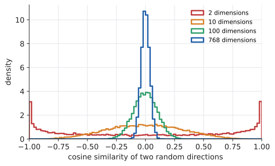
Why? The dot product of two random unit vectors is a sum of \(n\) small terms, each as likely to be positive as negative. Like a random walk, the positives and negatives mostly cancel. The typical size of such a sum, relative to the maximum possible, shrinks like \(1/\sqrt{n}\) (a fact you’ll be able to prove after Chapter 30). You can see it directly: Try it: Random cosines in 2D.
import numpy as np

rng = np.random.default_rng(42)
for d in [2, 3, 10, 100, 768, 4096]:
    X = rng.standard_normal((5000, d))
    Y = rng.standard_normal((5000, d))
    cos = np.sum(X * Y, axis=1) / (np.linalg.norm(X, axis=1) * np.linalg.norm(Y, axis=1))
    print(f"d={d:5d}  std of cos = {cos.std():.3f}   1/sqrt(d) = {1/np.sqrt(d):.3f}")
d= 2 std of cos = 0.709 1/sqrt(d) = 0.707 d= 3 std of cos = 0.576 1/sqrt(d) = 0.577 d= 10 std of cos = 0.310 1/sqrt(d) = 0.316 d= 100 std of cos = 0.103 1/sqrt(d) = 0.100 d= 768 std of cos = 0.036 1/sqrt(d) = 0.036 d= 4096 std of cos = 0.016 1/sqrt(d) = 0.016
This is good news and bad news. Good: in high dimensions there’s room for an enormous number of nearly independent directions, so a 768-dimensional space can encode many distinct concepts without them interfering. Bad: if your vectors are close to random, all similarities look alike, and "similar" becomes meaningless.
|
Three-dimensional intuition in high dimensions
|
|
Spin up the dimension
A slider sets the dimension \(n\) from 2 to 2000. The app draws 1000 random vector pairs and plots the histogram of their cosine similarities, with the curve narrowing as \(n\) grows. A second panel shows the distribution of distances from one random point to all others, so the learner can watch "nearest" and "farthest" converge. A third loads real sentence embeddings for the learner’s own sentences and compares their similarity scores against the random baseline. Try it: Spin up the dimension |
26.11. The cross product (three dimensions only)
26.11.1. The problem
A 3D model is made of triangles. To light a triangle with Lambert’s law, you need its normal vector: a vector perpendicular to the triangle’s surface. You have two edge vectors \(\mathbf{a}\) and \(\mathbf{b}\) lying in the triangle. How do you find a vector perpendicular to both?
26.11.2. The formula and its meaning
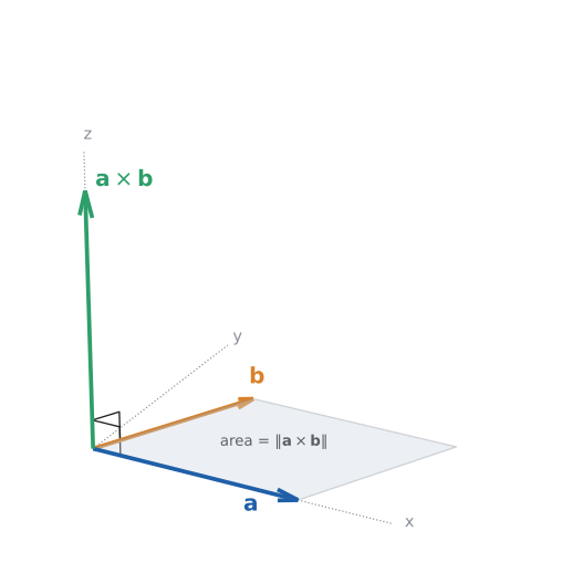
In three dimensions (and only there) there’s a product of two vectors that is a vector, perpendicular to both inputs:
A mnemonic for the pattern: for the first component, ignore the first entries and cross-multiply the second and third (\(a_2 b_3 - a_3 b_2\)); the other components cycle the indices \(1 \to 2 \to 3 \to 1\). (In Chapter 27 you’ll see it written as a determinant.)
Its geometric properties are what matter:
-
Direction: perpendicular to both \(\mathbf{a}\) and \(\mathbf{b}\), following the right-hand rule: point your right hand’s fingers along \(\mathbf{a}\), curl them towards \(\mathbf{b}\), and your thumb points along \(\mathbf{a}\times\mathbf{b}\).
-
Magnitude: \(\|\mathbf{a}\times\mathbf{b}\| = \|\mathbf{a}\|\,\|\mathbf{b}\|\sin\theta\), which is the area of the parallelogram the two vectors span. Parallel vectors (\(\theta = 0\)) give the zero vector.
-
Order matters: \(\mathbf{b}\times\mathbf{a} = -(\mathbf{a}\times\mathbf{b})\). Swapping flips the direction (it’s anticommutative).
|
Cross product
The cross product (vector product) \(\mathbf{a}\times\mathbf{b}\) of two 3D vectors is a 3D vector perpendicular to both, of length \(\|\mathbf{a}\|\,\|\mathbf{b}\|\sin\theta\), oriented by the right-hand rule. Contrast the dot product, which works in any dimension and returns a scalar involving \(\cos\theta\). In unit-vector form: \(\mathbf{i}\times\mathbf{j} = \mathbf{k}\), \(\mathbf{j}\times\mathbf{k} = \mathbf{i}\), \(\mathbf{k}\times\mathbf{i} = \mathbf{j}\). |
26.11.3. Worked example
Compute \((1, 2, 3)\times(4, 5, 6)\) and check the result. Try it: Cross product (1,2,3)×(4,5,6).
The parallelogram has area \(\sqrt{9 + 36 + 9} = \sqrt{54} \approx 7.35\), so the triangle with those two edges has half that, about 3.67. NumPy agrees: np.cross([1, 2, 3], [4, 5, 6]) returns array([-3, 6, -3]).
|
Only in 3D (and, oddly, 7D)
There is no cross product of two vectors in 2D, 4D, or 768D giving a vector perpendicular to both with these properties (a product of this kind exists only in 3 and 7 dimensions). In 2D, people often use the scalar \(a_1 b_2 - a_2 b_1\) ("2D cross product" in game code), which is the z-component of the 3D cross product of \((a_1, a_2, 0)\) and \((b_1, b_2, 0)\); its sign says whether \(\mathbf{b}\) is anticlockwise from \(\mathbf{a}\). In higher dimensions, the job of "area and orientation" is done by the determinant, which we meet in Chapter 27. |
26.12. Exercises: similarity and cross products
-
(Recognition) Two embeddings are normalised to length 1 and have dot product 0.82. What’s their cosine similarity, and what’s the Euclidean distance between them?
-
(Application) Compute the cosine similarity of the word-count vectors \((2, 0, 1)\) and \((1, 1, 1)\).
-
(Application) Find a normal vector to the triangle with corners \((0, 0, 0)\), \((1, 0, 0)\), \((0, 2, 2)\), and the triangle’s area.
-
(Problem solving) A search engine stores unnormalised TF-IDF vectors and ranks by dot product. A user complains that long, rambling pages always win. Explain the cause geometrically and propose a fix.
Answers
-
For unit vectors the dot product is the cosine similarity: 0.82. Distance: \(\sqrt{2 - 2(0.82)} = \sqrt{0.36} = 0.6\).
-
Dot product \(2 + 0 + 1 = 3\). Lengths \(\sqrt{5}\) and \(\sqrt{3}\). Cosine: \(3/\sqrt{15} \approx 0.775\).
-
Edges \(\mathbf{a} = (1, 0, 0)\), \(\mathbf{b} = (0, 2, 2)\). \(\mathbf{a}\times\mathbf{b} = (0\cdot 2 - 0\cdot 2,\ 0\cdot 0 - 1\cdot 2,\ 1\cdot 2 - 0\cdot 0) = (0, -2, 2)\). Check: dot with \(\mathbf{a}\) is 0, with \(\mathbf{b}\) is \(-4 + 4 = 0\). Parallelogram area \(\sqrt{8} = 2\sqrt{2}\), so the triangle’s area is \(\sqrt{2} \approx 1.41\).
-
\(\mathbf{q}\cdot\mathbf{d} = \|\mathbf{q}\|\,\|\mathbf{d}\|\cos\theta\). Long documents have large \(\|\mathbf{d}\|\), which inflates the score regardless of the angle (topic match). Fix: normalise document vectors to unit length at index time (rank by cosine similarity), or use a scoring function with explicit length normalisation such as BM25.
26.13. Summary
-
A vector has magnitude and direction. Picture it as an arrow (geometry) or store it as a list of components (computation); the two views always agree.
-
Vectors add component-wise (tip-to-tail), and scalar multiplication stretches, shrinks or flips them. Linear combinations of vectors span lines, planes, or whole spaces; checking whether a vector is in the span means solving a linear system.
-
Length is Pythagoras in any dimension: \(\|\mathbf{v}\| = \sqrt{\sum v_i^2}\). Normalising gives a unit vector; never normalise the zero vector.
-
The dot product \(\sum a_i b_i\) equals \(\|\mathbf{a}\|\,\|\mathbf{b}\|\cos\theta\) (from the law of cosines). Zero means orthogonal. It computes angles, work, projections, Lambert shading and reflections.
-
Projection onto \(\mathbf{b}\): \(\frac{\mathbf{a}\cdot\mathbf{b}}{\mathbf{b}\cdot\mathbf{b}}\mathbf{b}\), leaving a perpendicular residual.
-
Cosine similarity compares directions while ignoring length; for unit vectors it equals the dot product, and Euclidean distance ranks identically. Search engines, TF-IDF and embedding models all rank by it.
-
An embedding is the same mathematical object as \((3, 4)\), with more components. But high-dimensional space has surprises: random vectors are nearly orthogonal and distances concentrate.
-
The cross product (3D only) gives a vector perpendicular to two others, with length equal to their parallelogram’s area.
26.14. Interactive tools
Browser tools on the companion website that go with this chapter. Each example link in the chapter opens one of them with that example already set up.
26.15. Mastery check
-
Let \(\mathbf{u} = (1, -2, 2)\) and \(\mathbf{v} = (3, 0, 4)\). Compute \(\mathbf{u} + 2\mathbf{v}\), \(\|\mathbf{u}\|\), \(\|\mathbf{v}\|\), \(\mathbf{u}\cdot\mathbf{v}\), and the angle between \(\mathbf{u}\) and \(\mathbf{v}\).
-
Are \((2, 1)\) and \((-1, 2)\) orthogonal? Justify with one calculation.
-
Find the projection of \((4, 2)\) onto \((1, 1)\), and the unit vector in the direction of \((6, 8)\).
-
Write \((5, 4)\) as a linear combination of \((1, 1)\) and \((1, -1)\).
-
Derive \(\mathbf{a}\cdot\mathbf{b} = \|\mathbf{a}\|\,\|\mathbf{b}\|\cos\theta\) from the law of cosines, in three or four lines.
-
A surface has unit normal \(\mathbf{n} = (0, 0.6, 0.8)\) and the unit light direction is \(\mathbf{l} = (0, 0, 1)\). What fraction of full Lambert brightness does it receive? What if \(\mathbf{l} = (0, -0.8, -0.6)\)?
-
In a 1000-dimensional embedding space, about how large would you expect the cosine similarity of two unrelated random vectors to be? Why does this matter when interpreting a similarity score of 0.25?
-
Compute \((2, 0, 1)\times(1, 3, 0)\) and verify it’s perpendicular to both inputs.
Decision rule: All correct without hesitation → move on to Chapter 27. Stuck on 1–4 → reread Section 26.2, Section 26.4 and Section 26.5. Stuck on 5–6 → reread Section 26.6 and Section 26.7. Stuck on 7 → reread Section 26.9 and Section 26.10. Stuck on 8 → reread Section 26.11.
Mastery check answers
-
\(\mathbf{u} + 2\mathbf{v} = (1 + 6, -2 + 0, 2 + 8) = (7, -2, 10)\). \(\|\mathbf{u}\| = \sqrt{1 + 4 + 4} = 3\); \(\|\mathbf{v}\| = \sqrt{9 + 0 + 16} = 5\). \(\mathbf{u}\cdot\mathbf{v} = 3 + 0 + 8 = 11\). \(\cos\theta = 11/15 \approx 0.733\), so \(\theta \approx 42.8^\circ\).
-
\((2)(-1) + (1)(2) = 0\). Yes, orthogonal.
-
\(\frac{(4, 2)\cdot(1, 1)}{(1, 1)\cdot(1, 1)}(1, 1) = \frac{6}{2}(1, 1) = (3, 3)\). \(\|(6, 8)\| = 10\), so the unit vector is \((0.6, 0.8)\).
-
\(x(1, 1) + y(1, -1) = (5, 4)\) gives \(x + y = 5\), \(x - y = 4\). Adding: \(2x = 9\), \(x = 4.5\); then \(y = 0.5\). So \((5, 4) = 4.5(1, 1) + 0.5(1, -1)\).
-
\(\|\mathbf{a} - \mathbf{b}\|^2 = (\mathbf{a} - \mathbf{b})\cdot(\mathbf{a} - \mathbf{b}) = \|\mathbf{a}\|^2 + \|\mathbf{b}\|^2 - 2\,\mathbf{a}\cdot\mathbf{b}\). The law of cosines on the triangle with sides \(\mathbf{a}\), \(\mathbf{b}\), \(\mathbf{a} - \mathbf{b}\) gives \(\|\mathbf{a} - \mathbf{b}\|^2 = \|\mathbf{a}\|^2 + \|\mathbf{b}\|^2 - 2\|\mathbf{a}\|\,\|\mathbf{b}\|\cos\theta\). Equate and cancel: \(\mathbf{a}\cdot\mathbf{b} = \|\mathbf{a}\|\,\|\mathbf{b}\|\cos\theta\).
-
\(\mathbf{n}\cdot\mathbf{l} = 0 + 0 + 0.8 = 0.8\): 80% brightness (the surface is tilted about \(36.9^\circ\) from the light). With the second light, \(\mathbf{n}\cdot\mathbf{l} = 0 - 0.48 - 0.48 = -0.96 < 0\), so \(\max(0, \cdot) = 0\): the light is behind the surface, and it’s in shadow.
-
Typically about \(1/\sqrt{1000} \approx 0.03\) in size, almost always below 0.1. So 0.25 is far above chance for random vectors and is not "nearly unrelated" as 2D intuition might suggest. But real models' vectors aren’t random (they often share a common direction), so compare against other scores from the same model rather than reading 0.25 in isolation.
-
\((0\cdot 0 - 1\cdot 3,\ 1\cdot 1 - 2\cdot 0,\ 2\cdot 3 - 0\cdot 1) = (-3, 1, 6)\). Checks: \((-3, 1, 6)\cdot(2, 0, 1) = -6 + 0 + 6 = 0\); \((-3, 1, 6)\cdot(1, 3, 0) = -3 + 3 + 0 = 0\). ✓