Volume 1: Foundations to Precalculus · Part III: Geometry
Chapter 10. Coordinate Geometry
Draw a grid, give every point an address, and geometry becomes algebra. This chapter rebuilds the coordinate plane from scratch: distance and midpoint (Pythagoras in disguise), the three standard equations of a line, the slope test for perpendicular lines, circles by completing the square, a tour of the conic sections, and the four basic transformations written as coordinate rules. It ends where computer graphics begins: pixel grids with y pointing down, Bresenham’s line algorithm, bounding boxes, collision tests, and the difference between Euclidean and Manhattan distance.
Why it matters: every map app, sat-nav, CAD drawing, game, plotting library and GPS receiver works by storing positions as numbers and doing algebra on them. Once you can turn "is the phone within range of the mast?" or "where do these two roads cross?" into an equation, a computer can answer it a billion times a second.
10.1. Descartes' idea: geometry becomes algebra
10.1.1. The problem
Here is a classical geometry question: the three medians of a triangle (each joining a vertex to the midpoint of the opposite side) always meet at a single point. Why? With ruler-and-compass reasoning this takes a clever argument. With coordinates, it is a few lines of arithmetic: write the vertices as \((x_1, y_1)\), \((x_2, y_2)\), \((x_3, y_3)\), compute the point two-thirds of the way along each median, and notice that all three computations give the same answer, \(\left(\frac{x_1+x_2+x_3}{3}, \frac{y_1+y_2+y_3}{3}\right)\).
The reverse direction is just as powerful. The equation \(x^2 + y^2 = 25\) is a dry piece of algebra until you see that its solutions trace out a circle of radius 5. A picture makes the algebra obvious; algebra makes the picture precise.
10.1.2. Intuition
The idea, usually credited to René Descartes (and independently to Pierre de Fermat) in the 1630s, is to give every point an address: two numbers that say how far to go across and how far to go up from a fixed starting point. Once points are numbers:
-
a shape becomes an equation (the set of addresses that satisfy it);
-
a geometric question ("do these lines cross?") becomes an algebra question ("does this system have a solution?"), which you already know how to answer from Chapter 6;
-
a geometric operation ("rotate this triangle") becomes a formula applied to each address.
That third bullet is the foundation of every graphics engine, map application and CAD program ever written. A computer cannot see a triangle; it can only store and transform coordinates.
|
Analytic geometry
Analytic geometry (also coordinate geometry or Cartesian geometry) is the study of geometry using a coordinate system, so that geometric facts are proved and computed with algebra. It contrasts with synthetic geometry — Euclid’s style in Chapter 9 — which reasons directly from axioms and diagrams without numbers. |
|
The fly on the ceiling
A much-repeated story says Descartes, lying in bed, watched a fly crawl across the ceiling and realised he could describe its position at every moment by its distances from two walls. The story is almost certainly a legend, but the idea is right. Descartes published it in 1637 as La Géométrie, an appendix to his Discourse on the Method. The word Cartesian comes from his Latinised name, Renatus Cartesius. Fermat had the same idea at about the same time but did not publish it, a recurring theme in Fermat’s career. |
10.2. The Cartesian plane
10.2.1. Vocabulary and notation
Take two perpendicular number lines that cross at their zeros. The horizontal one is the x-axis, with positive numbers to the right; the vertical one is the y-axis, with positive numbers up. Every point \(P\) in the plane now has a unique address \((x, y)\): drop a perpendicular from \(P\) to each axis and read off the numbers.
|
Cartesian plane, axes, origin
The Cartesian plane (or coordinate plane, xy-plane) is the plane together with two perpendicular number lines, the axes. They meet at the origin, \(O = (0, 0)\). The horizontal axis is the x-axis; the vertical axis is the y-axis. |
|
Coordinates, ordered pair
A point’s coordinates are the ordered pair \((x, y)\). The first number, the x-coordinate (old name: abscissa), is the signed horizontal distance from the y-axis. The second, the y-coordinate (old name: ordinate), is the signed vertical distance from the x-axis. "Ordered" matters: \((2, 5)\) and \((5, 2)\) are different points. |
|
Quadrant
The axes cut the plane into four quadrants, numbered with Roman numerals anticlockwise starting from the top right: I (x positive, y positive), II (x negative, y positive), III (both negative), IV (x positive, y negative). Points that lie on an axis belong to no quadrant. |
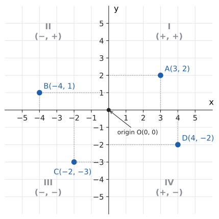
The anticlockwise numbering is not arbitrary: it is the direction in which a positive angle turns, which you will see again with the unit circle in Chapter 13.
|
(x, y), not (y, x) — and not (row, column)
The order is always "across, then up": x first. A helpful mnemonic is that you walk along the corridor before you go up the stairs. Programmers have an extra trap: two-dimensional arrays are indexed |
10.2.2. Exercises
-
Name the quadrant (or axis) containing each point: \((-3, 5)\), \((0, -4)\), \((2, -7)\), \((-1, -1)\).
-
A point has a negative x-coordinate and its y-coordinate is twice its x-coordinate. Which quadrant is it in?
-
The point \((a, b)\) is in quadrant II. Which quadrant contains \((b, a)\)? Which contains \((-a, b)\)?
Answers
-
\((-3, 5)\): quadrant II. \((0, -4)\): on the y-axis (no quadrant). \((2, -7)\): quadrant IV. \((-1, -1)\): quadrant III.
-
If \(x < 0\) then \(y = 2x < 0\) as well, so both coordinates are negative: quadrant III.
-
In quadrant II, \(a < 0\) and \(b > 0\). Then \((b, a)\) has positive x and negative y: quadrant IV. And \((-a, b)\) has \(-a > 0\) and \(b > 0\): quadrant I (it is the mirror image in the y-axis).
10.3. Distance and midpoint
10.3.1. The problem
A delivery drone sits at \((-2, 1)\) on a city map marked in kilometres; the customer is at \((4, 9)\). How far is the straight-line flight? And where should a relay station go if it must be exactly halfway?
10.3.2. Intuition
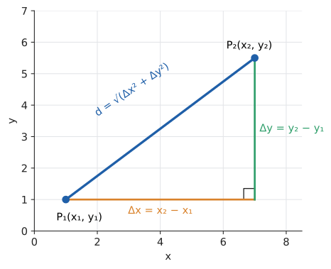
Any two points that are not level with each other are the ends of the hypotenuse of a right triangle whose other two sides run parallel to the axes. The horizontal leg is the change in \(x\); the vertical leg is the change in \(y\). Pythagoras (from Chapter 9) does the rest.
|
Delta notation
The Greek capital letter delta, \(\Delta\), is read "change in". So \(\Delta x = x_2 - x_1\) is the change in \(x\) going from the first point to the second. The subscripts \(x_1, x_2\) are just labels ("x of point 1", "x of point 2"), not powers or multiplications. |
10.3.3. Why it works
Let \(P_1 = (x_1, y_1)\) and \(P_2 = (x_2, y_2)\). The corner point \((x_2, y_1)\) makes a right angle, because one leg is horizontal and the other vertical. The legs have lengths \(|x_2 - x_1|\) and \(|y_2 - y_1|\). By Pythagoras:
Two pleasant consequences fall out. Because each difference is squared, it does not matter which point you call "1": \((x_1 - x_2)^2 = (x_2 - x_1)^2\). And if the points happen to be level (\(y_1 = y_2\)), the formula still works: it collapses to \(\sqrt{(x_2-x_1)^2} = |x_2 - x_1|\), which is the ordinary number-line distance.
|
Distance formula
The distance formula: the distance between \((x_1, y_1)\) and \((x_2, y_2)\) is \(d = \sqrt{(x_2 - x_1)^2 + (y_2 - y_1)^2}\). It is the Pythagorean theorem written in coordinates. This straight-line distance is called the Euclidean distance. |
The midpoint is even simpler. Halfway between two numbers on a line is their average; halfway between two points is the average in each coordinate separately, because moving halfway along the hypotenuse moves you halfway along each leg (the half-size triangle is similar to the full one, with scale factor \(\tfrac12\)).
|
Midpoint formula
The midpoint of the segment from \((x_1, y_1)\) to \((x_2, y_2)\) is \(M = \left(\dfrac{x_1 + x_2}{2}, \dfrac{y_1 + y_2}{2}\right)\), the coordinate-wise average. A segment (line segment) is the part of a line between two endpoints. |
10.3.4. The method
Input: two points \(P_1 = (x_1, y_1)\), \(P_2 = (x_2, y_2)\).
Steps:
-
Compute \(\Delta x = x_2 - x_1\) and \(\Delta y = y_2 - y_1\) (watch the signs when subtracting negatives).
-
Square each: \(\Delta x^2\), \(\Delta y^2\).
-
Add them, then take the square root: \(d = \sqrt{\Delta x^2 + \Delta y^2}\). Simplify the surd if exact form is wanted.
-
For the midpoint, average the x-coordinates and average the y-coordinates.
Output: the distance \(d\) and the midpoint \(M\).
10.3.5. Worked example
Drone at \(P_1 = (-2, 1)\), customer at \(P_2 = (4, 9)\).
Sanity check: the 6–8–10 triangle is the familiar 3–4–5 triangle doubled. And the distance from \((-2, 1)\) to the midpoint \((1, 5)\) is \(\sqrt{3^2 + 4^2} = 5\), exactly half. Good.
A second example with an unfriendly answer: from \((1, -3)\) to \((-4, 2)\).
10.3.6. Beyond the midpoint: any fraction of the way
What if you want the point one quarter of the way from \(P_1\) to \(P_2\)? The same similar-triangles argument says: move a quarter of \(\Delta x\) and a quarter of \(\Delta y\). In general, the point a fraction \(t\) of the way along is
At \(t = 0\) you are at \(P_1\); at \(t = 1\) at \(P_2\); at \(t = \tfrac12\) at the midpoint. This is the parametric form of a segment: the parameter \(t\) acts like time, and \(P(t)\) is where you are at that time. Equivalently, \(P(t) = (1-t)P_1 + tP_2\), a weighted average of the endpoints.
10.3.7. Choosing a method, and implementation
By hand, compute the differences first, then square; it keeps signs straight. In code, the standard library already knows the formula.
import math

def distance(p, q):
    """Euclidean distance between points p=(x1, y1) and q=(x2, y2)."""
    dx = q[0] - p[0]
    dy = q[1] - p[1]
    return math.sqrt(dx*dx + dy*dy)      # or math.hypot(dx, dy)

def midpoint(p, q):
    return ((p[0] + q[0]) / 2, (p[1] + q[1]) / 2)

def slope(p, q):
    dx = q[0] - p[0]
    if dx == 0:
        return None                      # vertical line: slope undefined
    return (q[1] - p[1]) / dx

P, Q = (-2, 1), (4, 9)
print(distance(P, Q), midpoint(P, Q), slope(P, Q))
print(math.dist(P, Q))                   # Python 3.8+, any dimension
10.0 (1.0, 5.0) 1.3333333333333333 10.0
math.hypot avoids overflow when \(\Delta x\) is enormous (squaring a \(10^{200}\) overflows a double; hypot rescales internally). math.dist works in any number of dimensions, which you will need in Section 10.10.
10.3.8. Failure modes
|
Three classic distance-formula slips
|
10.3.9. Where you’d use this
-
Navigation: on a small enough patch of the Earth that it looks flat, map coordinates plus the distance formula give straight-line distances. On a hiking map with a 1 km grid, a walk from grid position \((3.2, 7.5)\) to \((6.8, 2.7)\) is \(\sqrt{3.6^2 + 4.8^2} = \sqrt{12.96 + 23.04} = \sqrt{36} = 6\) km as the crow flies; the path will be longer, never shorter. (On a global scale you need spherical geometry; GPS uses 3D coordinates, see Section 10.10.)
-
Coordinate proofs: to prove a quadrilateral is a parallelogram, show its diagonals have the same midpoint; to prove a triangle is isosceles, show two side lengths are equal.
-
Machine learning: the k-nearest-neighbours classifier labels a new point by looking at the \(k\) training points with the smallest Euclidean distance to it.
|
Drag the triangle
Drag two points around the plane. The app draws the right triangle with legs \(\Delta x\) and \(\Delta y\), shows \(\Delta x^2 + \Delta y^2 = d^2\) updating live, and marks the point \(P(t)\) as you move a slider for \(t\) from 0 to 1. Try dragging one point across the other and watch \(\Delta x\) change sign while \(d\) stays positive. |
10.3.10. Exercises
-
Find the distance and midpoint of \((1, 2)\) and \((4, 6)\).
-
Find the distance and midpoint of \((-3, -1)\) and \((2, 11)\).
-
The midpoint of \(AB\) is \(M(3, -1)\) and \(A = (-2, 4)\). Find \(B\).
-
Find the point one quarter of the way from \((0, 0)\) to \((8, 12)\).
-
Show that the triangle with vertices \(A(1, 1)\), \(B(4, 3)\), \(C(2, 6)\) is a right isosceles triangle. Where is the right angle?
Answers
-
\(\Delta x = 3\), \(\Delta y = 4\), so \(d = \sqrt{9 + 16} = 5\). Midpoint \(\left(\frac{1+4}{2}, \frac{2+6}{2}\right) = (2.5, 4)\).
-
\(\Delta x = 2 - (-3) = 5\), \(\Delta y = 11 - (-1) = 12\), so \(d = \sqrt{25 + 144} = \sqrt{169} = 13\). Midpoint \(\left(\frac{-1}{2}, \frac{10}{2}\right) = (-0.5, 5)\).
-
\(M\) is the average, so \(B = 2M - A\) coordinate-wise: \(x_B = 2(3) - (-2) = 8\), \(y_B = 2(-1) - 4 = -6\). \(B = (8, -6)\).
-
With \(t = \tfrac14\): \((0 + \tfrac14 \cdot 8,\; 0 + \tfrac14 \cdot 12) = (2, 3)\).
-
Squared side lengths: \(AB^2 = 3^2 + 2^2 = 13\), \(BC^2 = (-2)^2 + 3^2 = 13\), \(AC^2 = 1^2 + 5^2 = 26\). Two sides are equal (isosceles) and \(AB^2 + BC^2 = 26 = AC^2\), so by the converse of Pythagoras the angle opposite \(AC\) — at \(B\) — is a right angle.
10.4. Slope revisited
You met slope in Chapter 5 as "rise over run". In coordinates it is
Three facts deserve restating now that we have the full plane.
|
Slope
The slope (or gradient) \(m\) of a non-vertical line is \(\frac{\Delta y}{\Delta x}\) between any two of its points — the change in \(y\) per unit increase in \(x\). Positive slope rises left-to-right, negative slope falls, zero slope is horizontal, and a vertical line has undefined slope (\(\Delta x = 0\), so you would divide by zero). |
Slope is the same between any two points on a line. Pick two different pairs of points on one line; the run–rise triangles they make are similar (equal angles, from parallel sides), so their ratios agree. This is why "the slope of a line" is meaningful at all, and it gives a quick collinearity test: three points lie on one line exactly when the slope from the first to the second equals the slope from the second to the third (or both are vertical).
Slope measures steepness as a tangent. If a line makes an angle \(\theta\) with the positive x-axis (its angle of inclination), then \(m = \tan\theta\). You will meet \(\tan\) properly in Chapter 13; for now, note that a 45° line has slope 1 and that slope grows without bound as the line approaches vertical.
Slope is a rate. If \(x\) is time in hours and \(y\) is distance in km, the slope is speed in km per hour. That reading — slope as rate of change — is exactly what calculus generalises to curves (Chapter 17).
Worked example: are \(A(1, 1)\), \(B(3, 4)\), \(C(7, 10)\) collinear? Try it: Check collinearity.
The slopes are equal and the segments share point \(B\), so yes. (Equal slopes alone are not enough: two parallel segments also have equal slopes. Sharing a point is what forces them onto one line.)
Where you’d use slope. Building regulations state slopes as ratios: a wheelchair ramp may be no steeper than 1:12 (US and UK guidance), so a 60 cm step needs at least \(0.6 \times 12 = 7.2\) m of ramp run. A road sign warning of a 10% hill means a slope of \(0.1\): 10 m up for every 100 m along, an angle of only about \(5.7^\circ\). In mechanics the slope of a distance–time graph is speed and the slope of a velocity–time graph is acceleration: a car going from 0 to 27 m/s in 9 s has an average acceleration of \(27/9 = 3\) m/s². In computing, the slope of a "requests served vs. time" graph is throughput, and the slope of a log of memory use is the leak rate you’re hunting.
10.5. Equations of lines
10.5.1. The problem
You know two points a road passes through, or one point and its gradient. You need a single equation that every point on the road satisfies — so a program can test whether a given point is on the road, find where it crosses another road, or draw it. Which equation, and in which form?
10.5.2. Intuition
A line is pinned down by two pieces of information: either two points, or one point and a slope. Each standard form of the equation is just one of those descriptions, written as an equation in \(x\) and \(y\).
10.5.3. Why it works: three forms
Point-slope form. Suppose the line has slope \(m\) and passes through \((x_1, y_1)\). A point \((x, y)\) (other than \((x_1, y_1)\) itself) is on the line exactly when the slope from \((x_1, y_1)\) to it equals \(m\):
The second line also holds at \((x_1, y_1)\) (both sides are zero), so it describes the whole line.
Slope-intercept form. Take the special point where the line crosses the y-axis, \((0, b)\). Point-slope gives \(y - b = m(x - 0)\), i.e.
Standard form. Move everything to one side and clear fractions:
Conventionally \(A, B, C\) are integers with no common factor and \(A \ge 0\). Standard form is the only one of the three that can describe a vertical line: \(x = 5\) is \(1\cdot x + 0 \cdot y = 5\). Its slope is \(-A/B\) (when \(B \ne 0\)); its intercepts are easy to read: set \(y = 0\) to get the x-intercept \(C/A\), set \(x = 0\) to get the y-intercept \(C/B\).
|
Forms of a linear equation
An intercept is where a graph crosses an axis: the x-intercept has \(y = 0\), the y-intercept has \(x = 0\). |
10.5.4. The method
Input: either two points \((x_1, y_1), (x_2, y_2)\), or a point \((x_1, y_1)\) and a slope \(m\).
Steps:
-
If given two points with \(x_1 = x_2\), stop: the line is vertical, \(x = x_1\).
-
If given two points, compute \(m = \frac{y_2 - y_1}{x_2 - x_1}\).
-
Write point-slope form \(y - y_1 = m(x - x_1)\) using either point.
-
To get slope-intercept form, expand and add \(y_1\) to both sides.
-
To get standard form, clear fractions (multiply by the denominators), then gather \(x\) and \(y\) terms on the left and the constant on the right; make \(A \ge 0\).
-
Check: substitute the other given point (or any known point) into your final equation.
Output: the line’s equation in the form you need.
10.5.5. Worked examples
Two points. Line through \((1, 2)\) and \((3, 8)\).
Check with \((3, 8)\): \(3(3) - 1 = 8\). Correct.
Point and fractional slope. Through \((-4, 1)\) with slope \(-\tfrac{2}{3}\).
Slope-intercept is \(y = -\tfrac23 x - \tfrac53\). Check: \(2(-4) + 3(1) = -8 + 3 = -5\). Correct.
From standard form to a sketch. \(4x - 3y = 12\). Intercepts: \(y = 0 \Rightarrow x = 3\); \(x = 0 \Rightarrow y = -4\). Plot \((3, 0)\) and \((0, -4)\) and join them. Slope: \(-A/B = -4/(-3) = \tfrac43\).
10.5.6. Choosing a form
| Form | Use it when… | Weakness |
|---|---|---|
\(y = mx + b\) |
graphing, reading off slope and intercept, computing \(y\) from \(x\) |
cannot express vertical lines |
\(y - y_1 = m(x - x_1)\) |
building the equation from a point and a slope (the fastest route) |
not unique: each point gives a different-looking equation |
\(Ax + By = C\) |
solving systems (Chapter 6), integer arithmetic, vertical lines, quick intercepts |
slope not visible at a glance |
Rule of thumb: build in point-slope, present in slope-intercept for graphing or in standard form for systems and code.
10.5.7. Where you’d use this
-
Deciding between deals. A gym charges $8 per visit, or $30 a month plus $2 per visit. Monthly cost is \(y = 8v\) or \(y = 30 + 2v\) for \(v\) visits; the lines cross where \(8v = 30 + 2v\), i.e. \(v = 5\). Five visits a month costs $40 either way; more than five and the membership wins. Phone plans, car hire and electricity tariffs (standing charge plus a rate per kWh) are all lines with an intercept and a slope.
-
Unit conversion. Fahrenheit is a linear function of Celsius. Two known points, \((0, 32)\) (water freezes) and \((100, 212)\) (water boils), give slope \(180/100 = 1.8\) and the line \(F = 1.8C + 32\).
-
Calibrating a sensor. A temperature sensor outputs 0.50 V at 20 °C and 1.30 V at 100 °C. Its slope is \((1.30 - 0.50)/(100 - 20) = 0.01\) V per °C, so a reading of 0.82 V means \(T = 20 + (0.82 - 0.50)/0.01 = 52\) °C. Every two-point calibration in a lab or in firmware is "the line through two points". Hooke’s law for a spring (\(F = kx\)) is the same idea with intercept zero.
-
Computing. Lookup tables (tax bands, colour ramps, game difficulty curves) store a few points and draw straight lines between them; the line through two points is how a program fills the gaps.
|
Horizontal and vertical are easy to swap by accident
\(y = 3\) is a horizontal line (every point has height 3, any \(x\)). \(x = 3\) is a vertical line. Horizontal lines have slope 0; vertical lines have no slope — "undefined", not zero, and not infinity in the sense of a number you can compute with. If a program computes |
10.5.8. Exercises
-
Find the slope of the line through \((-1, 4)\) and \((3, -4)\), and write the line in all three forms.
-
Convert \(4x - 3y = 12\) to slope-intercept form and state both intercepts.
-
Which form would you choose to describe the line through \((2, -1)\) and \((2, 6)\), and why?
-
A taxi charges a fixed fee plus a rate per km. A 3 km trip costs $8.50 and an 8 km trip costs $16. Write cost \(y\) as a function of distance \(x\) and interpret the slope and intercept.
Answers
-
\(m = \frac{-4 - 4}{3 - (-1)} = \frac{-8}{4} = -2\). Point-slope: \(y - 4 = -2(x + 1)\). Expand: \(y - 4 = -2x - 2\), so slope-intercept \(y = -2x + 2\). Standard: \(2x + y = 2\). Check \((3, -4)\): \(6 - 4 = 2\). Correct.
-
\(-3y = -4x + 12\), divide by \(-3\): \(y = \tfrac43 x - 4\). x-intercept \((3, 0)\), y-intercept \((0, -4)\).
-
Both points have \(x = 2\), so the line is vertical: \(x = 2\). Only standard form (\(1x + 0y = 2\)) can express it; slope-intercept cannot.
-
Points \((3, 8.50)\) and \((8, 16)\). \(m = \frac{16 - 8.5}{8 - 3} = \frac{7.5}{5} = 1.5\). Point-slope: \(y - 8.5 = 1.5(x - 3)\), so \(y = 1.5x + 4\). Slope: $1.50 per km. Intercept: a $4 fixed fee (the cost of a 0 km trip).
10.6. Parallel and perpendicular lines
10.6.1. The problem
A city planner wants a new street through a given point running parallel to an existing avenue, and a footpath from a building that meets the avenue at a right angle (the shortest route). Given the avenue’s equation, what are the slopes of these new lines?
10.6.2. Intuition
Parallel lines never meet, so neither can be steeper than the other: they have equal slopes (and different intercepts — equal slope and equal intercept would be the same line). Vertical lines are all parallel to each other.
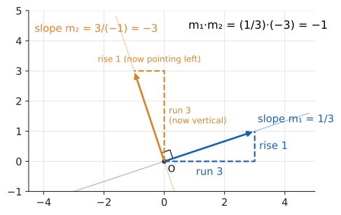
Perpendicular lines are subtler. Take the run–rise triangle of a line with slope \(m_1 = \tfrac13\): run 3, rise 1. Now rotate the whole picture by 90° anticlockwise. The run of 3 becomes a vertical rise of 3; the rise of 1 becomes a horizontal step of 1 to the left. The rotated line therefore has slope \(\frac{3}{-1} = -3\). The slope flipped upside down and changed sign.
10.6.3. Why it works: two derivations
By rotation. A line with slope \(m_1 = \frac{a}{b}\) has direction "run \(b\), rise \(a\)", i.e. moves from the origin to \((b, a)\). Rotating a point 90° anticlockwise about the origin sends \((x, y)\) to \((-y, x)\) (we justify this rule in Section 10.9). So the perpendicular direction is \((-a, b)\), with slope \(m_2 = \frac{b}{-a} = -\frac{b}{a}\). Hence
By Pythagoras. Shift both lines so they pass through the origin (that changes neither slope nor angle): \(y = m_1 x\) and \(y = m_2 x\). They contain the points \(A = (1, m_1)\) and \(B = (1, m_2)\). The angle at \(O\) is a right angle exactly when \(OA^2 + OB^2 = AB^2\) (Pythagoras and its converse, Chapter 9):
Every step is reversible, so the condition is both necessary and sufficient.
|
Parallel and perpendicular slopes
Two non-vertical lines with slopes \(m_1, m_2\) are
The reciprocal of \(\frac{a}{b}\) is \(\frac{b}{a}\) (flip it); the negative reciprocal flips and changes sign. Special case: horizontal (\(m = 0\)) and vertical lines are perpendicular, but the product rule cannot express this since a vertical slope does not exist. |
10.6.4. The method
Input: a line \(L\) and a point \(P = (x_1, y_1)\).
Steps:
-
Find the slope \(m\) of \(L\) (rearrange to \(y = mx + b\), or use \(m = -A/B\) from standard form).
-
Parallel: use slope \(m\). Perpendicular: use \(-1/m\) (if \(m = 0\), the perpendicular is the vertical line \(x = x_1\); if \(L\) is vertical, the perpendicular is horizontal, \(y = y_1\)).
-
Write point-slope form through \(P\) and simplify.
-
Check: \(P\) satisfies the new equation, and the slope product is \(-1\) (perpendicular) or the slopes match (parallel).
Output: the equation of the required line.
10.6.5. Worked examples
Perpendicular through a point. Find the line through \((4, 1)\) perpendicular to \(y = \tfrac23 x + 1\).
Check: \(-\tfrac32(4) + 7 = 1\); \(\tfrac23 \cdot (-\tfrac32) = -1\). In standard form, \(3x + 2y = 14\).
Perpendicular bisector. The perpendicular bisector of a segment is the line through its midpoint at right angles to it. Every point on it is equally far from both endpoints, which makes it the answer to "where are all the places equally close to A and B?". For \(A(1, 2)\) and \(B(7, 6)\):
Check: \((0, 10)\) is on this line. Its squared distance to \(A\) is \(1 + 64 = 65\); to \(B\), \(49 + 16 = 65\). Equal, as promised.
10.6.6. Distance from a point to a line
The shortest path from a point to a line is the perpendicular one. Doing the perpendicular construction in general (find the perpendicular through the point, intersect it with the line, apply the distance formula) gives a compact formula: the distance from \((x_0, y_0)\) to the line \(Ax + By = C\) is
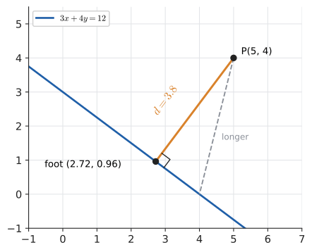
Example: from \((5, 4)\) to \(3x + 4y = 12\), \(d = \frac{|15 + 16 - 12|}{\sqrt{9 + 16}} = \frac{19}{5} = 3.8\). To confirm by the long route: the perpendicular through \((5, 4)\) has direction \((3, 4)\), so its points are \((5 + 3t, 4 + 4t)\). Substituting into the line, \(3(5 + 3t) + 4(4 + 4t) = 12 \Rightarrow 31 + 25t = 12 \Rightarrow t = -0.76\), giving foot \((2.72, 0.96)\). The distance is \(|t| \cdot \sqrt{3^2 + 4^2} = 0.76 \times 5 = 3.8\). The two routes agree. Notice the numerator is just \(|F(x_0, y_0)|\), the side-of-line test from the previous CS sidebar: its sign says which side, and divided by \(\sqrt{A^2+B^2}\) its size says how far.
10.6.7. Where you’d use this
-
Voronoi diagrams. Given several cell towers, which tower is nearest to each location? The boundary between two towers' regions is the perpendicular bisector of the segment joining them. Voronoi diagrams built from these bisectors appear in mobile networks, epidemiology (John Snow’s 1854 cholera map is essentially one), and nearest-neighbour search.
-
Circumcentre. The perpendicular bisectors of a triangle’s three sides meet at one point, equidistant from all three vertices — the centre of the circle through them.
-
Shortest connection. The footpath in our opening problem runs along the perpendicular from the building to the avenue; its length is the point-to-line distance.
10.6.8. Exercises
-
Find the line through \((2, 1)\) parallel to \(y = -x + 7\).
-
Find the line through the origin perpendicular to \(2x + 5y = 10\).
-
Find the perpendicular bisector of the segment from \((-1, 3)\) to \((5, -1)\), and verify one point on it is equidistant from both endpoints.
-
Find the distance from \((1, -2)\) to the line \(5x - 12y = 3\).
-
Are the lines \(3x - 4y = 7\) and \(8x + 6y = 1\) parallel, perpendicular, or neither?
Answers
-
Slope \(-1\). \(y - 1 = -(x - 2)\), so \(y = -x + 3\).
-
Given slope \(-A/B = -\tfrac25\); perpendicular slope \(\tfrac52\). Through the origin: \(y = \tfrac52 x\).
-
Midpoint \((2, 1)\). Segment slope \(\frac{-1 - 3}{5 - (-1)} = -\tfrac23\); perpendicular slope \(\tfrac32\). \(y - 1 = \tfrac32(x - 2)\), so \(y = \tfrac32 x - 2\). Check with \((0, -2)\): squared distance to \((-1, 3)\) is \(1 + 25 = 26\); to \((5, -1)\) is \(25 + 1 = 26\). Equal.
-
\(d = \frac{|5(1) - 12(-2) - 3|}{\sqrt{25 + 144}} = \frac{|5 + 24 - 3|}{13} = \frac{26}{13} = 2\).
-
Slopes: \(-A/B = \tfrac34\) and \(-\tfrac86 = -\tfrac43\). Product \(\tfrac34 \cdot (-\tfrac43) = -1\): perpendicular.
10.7. Circles
10.7.1. The problem
A phone mast has a range of 5 km and stands at \((3, -2)\) on a map grid. Which grid points get signal? Equally often you are handed the problem the other way round: an equation like \(x^2 + y^2 - 6x + 4y - 12 = 0\) comes out of some calculation, and you need to recognise it as a circle and find its centre and radius.
10.7.2. Intuition and derivation
A circle is the set of all points at a fixed distance (the radius) from a fixed point (the centre). That definition is the distance formula. A point \((x, y)\) lies on the circle with centre \((h, k)\) and radius \(r > 0\) exactly when
So the mast’s coverage boundary is \((x - 3)^2 + (y + 2)^2 = 25\), and the points with signal are those with \((x - 3)^2 + (y + 2)^2 \le 25\). Note the sign flip: centre \(k = -2\) appears as \((y - (-2))^2 = (y + 2)^2\).
|
Equation of a circle
The standard form (or centre–radius form) of a circle with centre \((h, k)\) and radius \(r\) is \((x - h)^2 + (y - k)^2 = r^2\). The circle centred at the origin is \(x^2 + y^2 = r^2\); with \(r = 1\) it is the unit circle, the star of Chapter 13. Expanding standard form gives the general form \(x^2 + y^2 + Dx + Ey + F = 0\). |
10.7.3. The method: completing the square
Expanding \((x - 3)^2 + (y + 2)^2 = 25\) gives \(x^2 - 6x + 9 + y^2 + 4y + 4 = 25\), i.e. \(x^2 + y^2 - 6x + 4y - 12 = 0\). To go backwards — from the general form to centre and radius — you complete the square in \(x\) and in \(y\) separately, exactly as in Chapter 8.
Input: an equation with \(x^2\) and \(y^2\) terms having equal coefficients and no \(xy\) term.
Steps:
-
If the \(x^2\) and \(y^2\) coefficients are not 1, divide the whole equation by that coefficient.
-
Group the \(x\) terms, group the \(y\) terms, and move the constant to the right.
-
For the \(x\) group \(x^2 + Dx\), add \((D/2)^2\) to both sides; it becomes \((x + D/2)^2\). Do the same for \(y\).
-
Read off: centre \((h, k) = (-D/2, -E/2)\), and the right-hand side is \(r^2\).
-
If the right-hand side is positive, \(r\) is its square root. If it is zero, the "circle" is the single point \((h, k)\). If it is negative, there are no points at all.
Output: centre \((h, k)\) and radius \(r\), or a note that the equation is degenerate.
10.7.4. Worked example
\(x^2 + y^2 - 6x + 4y - 12 = 0\).
Centre \((3, -2)\), radius \(\sqrt{25} = 5\): the phone mast again.
A version with a leading coefficient: \(2x^2 + 2y^2 - 4x + 12y - 30 = 0\).
import math

def circle_from_general(D, E, F):
    """x^2 + y^2 + Dx + Ey + F = 0  ->  (h, k, r), or None if no real circle."""
    h, k = -D / 2, -E / 2
    r_squared = h*h + k*k - F
    if r_squared < 0:
        return None                      # no points at all
    return h, k, math.sqrt(r_squared)

print(circle_from_general(-6, 4, -12))  # x^2+y^2-6x+4y-12=0
print(circle_from_general(2, 2, 10))
(3.0, -2.0, 5.0) None
The second call is \(x^2 + y^2 + 2x + 2y + 10 = 0\), i.e. \((x+1)^2 + (y+1)^2 = -8\): a sum of squares cannot be negative, so no point satisfies it.
10.7.5. Lines meeting circles, and tangents
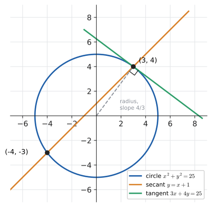
Where does the line \(y = x + 1\) meet the circle \(x^2 + y^2 = 25\)? Substitute the line into the circle — the substitution method of Chapter 6: Try it: Line meets circle, discriminant.
So \(x = 3, y = 4\) or \(x = -4, y = -3\): two crossing points. In general, the resulting quadratic’s discriminant (Chapter 8) tells the story: positive means the line cuts the circle twice (a secant), zero means it touches once (a tangent), negative means it misses.
A tangent to a circle is perpendicular to the radius at the point of contact (Chapter 9). That turns "find the tangent" into a slope problem. Tangent to \(x^2 + y^2 = 25\) at \((3, 4)\): the radius has slope \(\tfrac43\), so the tangent has slope \(-\tfrac34\), and \(y - 4 = -\tfrac34(x - 3)\), which simplifies to \(3x + 4y = 25\). Try it: See the tangent touch.
|
Not every x² + y² equation is a circle
|
10.7.6. Where you’d use this
-
Delivery and coverage zones. A pizza shop at map position \((2, 1)\) (in km) delivers within 3 km. Do you, at \((4, 3)\), qualify? \((4-2)^2 + (3-1)^2 = 8 \le 9 = 3^2\): yes, just. Phone masts, Wi-Fi access points, fire-station response areas and "stores near me" searches all run this inequality.
-
Positioning by trilateration. If you know you are 5 km from beacon \(A(0, 0)\) and 5 km from beacon \(B(6, 0)\), you are on both circles \(x^2 + y^2 = 25\) and \((x - 6)^2 + y^2 = 25\). Subtracting the equations kills the squares: \(x^2 - (x - 6)^2 = 0\), so \(12x - 36 = 0\) and \(x = 3\); then \(y^2 = 16\), so \(y = \pm 4\). A third beacon picks between \((3, 4)\) and \((3, -4)\). GPS does the same with spheres in 3D (plus one more satellite to fix the receiver’s clock error), and indoor positioning does it with Wi-Fi or Bluetooth signal strengths.
-
Engineering and graphics. Gear teeth, cams, roundabouts and railway curves are laid out from circle equations; a CNC machine cutting an arc and a font renderer drawing a rounded corner both need centre and radius. Tangent lines matter wherever a straight piece must join a curve smoothly: a road leaving a roundabout, a belt leaving a pulley.
10.7.7. Exercises
-
Write the equation of the circle with centre \((-1, 4)\) and radius 3.
-
Find the centre and radius of \(x^2 + y^2 + 8x - 2y + 8 = 0\).
-
Is the point \((4, 4)\) inside, on, or outside the circle \(x^2 + y^2 - 6x + 4y - 12 = 0\)?
-
Find the tangent to \(x^2 + y^2 = 13\) at \((2, -3)\).
-
Find where the line \(y = 7 - x\) meets the circle \(x^2 + y^2 = 25\). Try it: Check your answer.
Answers
-
\((x + 1)^2 + (y - 4)^2 = 9\).
-
\((x^2 + 8x + 16) + (y^2 - 2y + 1) = -8 + 16 + 1 = 9\), so \((x + 4)^2 + (y - 1)^2 = 9\): centre \((-4, 1)\), radius 3.
-
In standard form the circle is \((x - 3)^2 + (y + 2)^2 = 25\). At \((4, 4)\): \(1^2 + 6^2 = 37 > 25\), so outside.
-
Radius slope \(\frac{-3}{2}\); tangent slope \(\frac{2}{3}\). \(y + 3 = \tfrac23(x - 2)\) → \(3y + 9 = 2x - 4\) → \(2x - 3y = 13\). Check: \(4 + 9 = 13\). Correct.
-
\(x^2 + (7 - x)^2 = 25\) → \(2x^2 - 14x + 49 = 25\) → \(x^2 - 7x + 12 = 0\) → \((x - 3)(x - 4) = 0\). Points \((3, 4)\) and \((4, 3)\).
10.8. Conic sections
10.8.1. The problem
Why are satellite dishes and car headlights shaped the way they are? Why do planets trace ovals and some comets swing past the Sun once and never return? And what do all of those have to do with the circle you just met?
10.8.2. Intuition: slicing a cone
Take a double cone (two ice-cream cones joined at their tips) and slice it with a plane. Depending on the tilt of the slice you get exactly four kinds of curve, the conic sections: Try it: Slice the cone yourself.
-
slice straight across: a circle;
-
tilt a little: a closed oval, an ellipse;
-
tilt until the plane is parallel to the side of the cone: an open U-shape, a parabola;
-
tilt further still, cutting both halves of the cone: a two-piece curve, a hyperbola.
In coordinates, every conic is the graph of a second-degree equation \(Ax^2 + Bxy + Cy^2 + Dx + Ey + F = 0\). Lines are degree 1; conics are the next step up.
|
Conic section
A conic section (conic) is a curve obtained by intersecting a plane with a double cone: circle, ellipse, parabola or hyperbola. Each (except the circle) can also be defined by a focus (a fixed point; plural foci) and a directrix (a fixed line). The vertex is the point where a parabola turns; the axis of symmetry is the line it is mirror-symmetric about. |
10.8.3. Parabola: equal distances to a point and a line
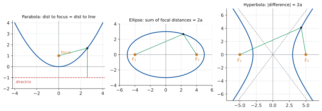
A parabola is the set of points equally far from a focus and a directrix. Put the focus at \((0, p)\) and the directrix at \(y = -p\). For a point \((x, y)\), the distance to the focus is \(\sqrt{x^2 + (y - p)^2}\) and the distance to the line is \(|y + p|\). Setting them equal:
So \(y = \frac{x^2}{4p}\): the familiar parabola of Chapter 8, now with geometric meaning attached to its coefficient. For \(y = \tfrac14 x^2\), \(4p = 4\), so the focus is \((0, 1)\) and the directrix is \(y = -1\). If \(p < 0\) the parabola opens downward. Try it: Focus and directrix of y = x²/4.
The reflective property explains the dish: every ray arriving parallel to the axis bounces off a parabolic mirror straight through the focus. Put the receiver at the focus and it collects all the signal; put a bulb there and the headlight sends out a parallel beam. Try it: Watch the rays reflect.
10.8.4. Ellipse and hyperbola: sums and differences
An ellipse is the set of points whose distances to two foci \(F_1, F_2\) add up to a constant \(2a\). (Pin a loop of string at two points and trace around with a pencil.) With foci \((\pm c, 0)\), the algebra — the same square-twice routine as the parabola, just longer — gives
\(a\) is the semi-major axis (half the longest width), \(b\) the semi-minor axis. When \(c = 0\) the foci merge, \(a = b\), and you get a circle.
A hyperbola is the set of points whose distances to two foci differ by a constant \(2a\) (in absolute value). With foci \((\pm c, 0)\):
with asymptotes \(y = \pm \frac{b}{a} x\) — lines the branches approach but never reach.
|
Eccentricity
The eccentricity \(e\) of a conic is the ratio (distance to focus) / (distance to directrix), which is the same for every point on it. \(e = 0\): circle. \(0 < e < 1\): ellipse (for the standard ellipse, \(e = c/a\)). \(e = 1\): parabola. \(e > 1\): hyperbola. One number classifies them all. |
Worked example: identify each conic and its key features.
-
\(\frac{x^2}{25} + \frac{y^2}{9} = 1\): ellipse with \(a = 5\), \(b = 3\), \(c = \sqrt{25 - 9} = 4\). Foci \((\pm 4, 0)\), eccentricity \(\tfrac45 = 0.8\). Check with the point \((0, 3)\): its distances to the foci are each \(\sqrt{16 + 9} = 5\), summing to \(10 = 2a\). Try it: This ellipse from its focus.
-
\(\frac{x^2}{9} - \frac{y^2}{16} = 1\): hyperbola, \(a = 3\), \(b = 4\), \(c = \sqrt{9 + 16} = 5\). Foci \((\pm 5, 0)\), asymptotes \(y = \pm\tfrac43 x\). Check with the vertex \((3, 0)\): distances 8 and 2, difference \(6 = 2a\). Try it: This hyperbola from its focus.
-
\(x^2 = -12y\): parabola, \(4p = -12\), \(p = -3\). Opens downward; focus \((0, -3)\), directrix \(y = 3\). Try it: This parabola from its focus.
10.8.5. Where you’d use this
-
Orbits. Kepler’s first law: planets move on ellipses with the Sun at one focus. Earth’s orbit has \(e \approx 0.017\) (nearly a circle); Halley’s comet has \(e \approx 0.97\). The focus is not at the centre, so the distance to the Sun varies: with semi-major axis \(a \approx 149.6\) million km, the closest approach is \(a(1 - e) \approx 147.1\) million km (early January) and the farthest \(a(1 + e) \approx 152.1\) million km (early July). Seasons come from the tilt of Earth’s axis, not this 3% difference. An object moving faster than escape velocity follows a hyperbola and leaves forever.
-
Reflectors. Parabolic dishes, telescope mirrors, solar cookers. Elliptical "whispering galleries" carry a whisper from one focus to the other; lithotripsy machines focus shock waves on a kidney stone the same way.
-
Positioning. If two radio stations transmit simultaneously and you measure the difference in arrival times, you know the difference of your distances to them: you are on a hyperbola with the stations as foci. Two such hyperbolas pin you down. This was the LORAN navigation system, and the same time-difference idea underlies GPS and microphone-array sound location.
-
Projectiles. Ignoring air resistance, a thrown ball follows a parabola.
|
Apollonius and Kepler
Apollonius of Perga (c. 200 BCE) wrote eight books on conics and gave us the names ellipse ("falling short"), parabola ("thrown alongside", i.e. exactly matching) and hyperbola ("thrown beyond", i.e. exceeding) — originally describing how an area compared with another in his constructions. The same roots give "ellipsis" (words left out), "parable" and "hyperbole" (exaggeration). For 1800 years conics were a purely geometric curiosity, until Kepler discovered in 1609 that the planets move on ellipses. |
|
Focus and directrix playground
Place a focus and a directrix, then drag a slider for eccentricity \(e\). The app plots every point whose focus-distance is \(e\) times its directrix-distance. Watch the ellipse stretch as \(e \to 1\), snap into a parabola at \(e = 1\), and split into a hyperbola beyond. A second mode slices a 3D cone with a tiltable plane. |
10.8.6. Exercises
-
Identify each conic and give its foci: (a) \(\frac{x^2}{16} + \frac{y^2}{9} = 1\); (b) \(y = \frac{x^2}{8}\); (c) \(\frac{x^2}{4} - \frac{y^2}{5} = 1\).
-
A satellite dish is a parabola in cross-section, 60 cm across and 9 cm deep. How far from the vertex should the receiver go? Try it: Check your answer.
-
Find the equation of the ellipse with foci \((\pm 3, 0)\) and major axis of length 10.
Answers
-
(a) Ellipse, \(a = 4\), \(b = 3\), \(c = \sqrt{16 - 9} = \sqrt7\); foci \((\pm\sqrt7, 0)\). (b) Parabola, \(4p = 8\), \(p = 2\); focus \((0, 2)\), directrix \(y = -2\). (c) Hyperbola, \(a = 2\), \(b = \sqrt5\), \(c = \sqrt{4 + 5} = 3\); foci \((\pm 3, 0)\), asymptotes \(y = \pm\frac{\sqrt5}{2}x\).
-
Model as \(x^2 = 4py\) with the vertex at the origin. The rim is at \((30, 9)\): \(900 = 4p \cdot 9 = 36p\), so \(p = 25\). The receiver goes 25 cm from the vertex along the axis.
-
\(2a = 10 \Rightarrow a = 5\); \(c = 3\); \(b^2 = a^2 - c^2 = 16\). \(\frac{x^2}{25} + \frac{y^2}{16} = 1\).
10.9. Transformations as coordinate rules
10.9.1. The problem
A game character is drawn as a list of vertex coordinates. The player presses "turn left": every vertex must rotate 90° about the character’s centre. Then the camera zooms, the level scrolls, a mirror-image enemy appears. Each of these is a rule that takes a point’s coordinates and produces new ones. What are the rules?
10.9.2. Intuition
In Chapter 9 you met congruence (same shape and size) and similarity (same shape, scaled). Transformations are the moves that produce congruent or similar copies. On the coordinate plane each move is a function from points to points, written \((x, y) \mapsto (x', y')\) — read "\((x, y)\) maps to \((x', y')\)". The original is the pre-image; the result is the image, conventionally labelled with primes (\(A \mapsto A'\)).
|
Transformation, image, isometry
A transformation of the plane is a rule that sends every point to a new point. The image of \(A\) is written \(A'\) ("A prime"). An isometry or rigid motion preserves all distances (and hence angles and areas): translations, reflections and rotations are isometries, and they produce congruent figures. A dilation scales all distances by the same factor and produces similar figures. |
10.9.3. The four basic rules
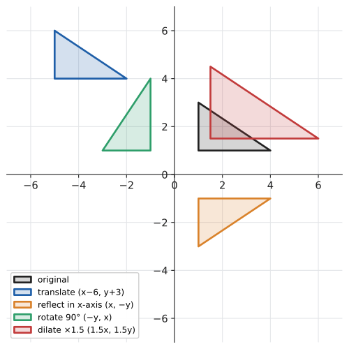
Translation (slide) by \(a\) across and \(b\) up: \((x, y) \mapsto (x + a, y + b)\). Every point moves by the same vector \((a, b)\).
Reflection (mirror):
-
in the x-axis: \((x, y) \mapsto (x, -y)\) — the height flips sign;
-
in the y-axis: \((x, y) \mapsto (-x, y)\);
-
in the line \(y = x\): \((x, y) \mapsto (y, x)\) — the coordinates swap;
-
in the origin (point reflection): \((x, y) \mapsto (-x, -y)\).
Rotation about the origin, anticlockwise:
-
by 90°: \((x, y) \mapsto (-y, x)\);
-
by 180°: \((x, y) \mapsto (-x, -y)\) (the same as the point reflection);
-
by 270° (= 90° clockwise): \((x, y) \mapsto (y, -x)\).
Dilation (scaling) about the origin with scale factor \(k\): \((x, y) \mapsto (kx, ky)\). \(|k| > 1\) enlarges, \(0 < |k| < 1\) shrinks; a negative \(k\) also rotates by 180°.
10.9.4. Why the rotation rule works
Think of \((x, y)\) as "\(x\) steps along the x-direction \((1, 0)\), plus \(y\) steps along the y-direction \((0, 1)\)". A 90° anticlockwise turn sends the direction \((1, 0)\) (east) to \((0, 1)\) (north), and sends \((0, 1)\) (north) to \((-1, 0)\) (west). Rotating the whole picture rotates the step directions and keeps the step counts:
The same argument works for any angle \(\theta\): east goes to \((\cos\theta, \sin\theta)\) and north to \((-\sin\theta, \cos\theta)\), so
You will meet \(\cos\) and \(\sin\) in Chapter 13; check that \(\theta = 90^\circ\) (\(\cos = 0\), \(\sin = 1\)) gives back \((-y, x)\). The idea "a transformation is determined by where it sends the two basic directions" is exactly what a matrix records. The 90° rotation is the matrix \(\begin{pmatrix} 0 & -1 \\ 1 & 0 \end{pmatrix}\), and composing transformations becomes multiplying matrices — the whole subject of Chapter 27.
10.9.5. The method: transforming about any point
The rotation and dilation rules above use the origin as their fixed centre. To rotate or scale about another point, move that point to the origin, transform, and move back.
Input: a point \(P = (x, y)\), a centre \(C = (c_1, c_2)\), and a rotation (or dilation) rule about the origin.
Steps:
-
Translate so the centre is at the origin: \((u, v) = (x - c_1, y - c_2)\).
-
Apply the origin-centred rule to \((u, v)\), giving \((u', v')\).
-
Translate back: \(P' = (u' + c_1, v' + c_2)\).
-
Check (rotation): \(P\) and \(P'\) are the same distance from \(C\).
Output: the image \(P'\).
10.9.6. Worked examples
A triangle, rotated. Rotate \(A(1, 1)\), \(B(4, 1)\), \(C(1, 3)\) by 90° anticlockwise about the origin with \((x, y) \mapsto (-y, x)\): \(A' = (-1, 1)\), \(B' = (-1, 4)\), \(C' = (-3, 1)\). Check a side: \(AB = 3\), and \(A'B' = \sqrt{0^2 + 3^2} = 3\). Distances preserved, as an isometry must. Try it: Triangle rotated 90°; Rotate P(5,3) about C(2,1).
About another centre. Rotate \(P(5, 3)\) by 90° anticlockwise about \(C(2, 1)\).
Check: \(CP = \sqrt{3^2 + 2^2} = \sqrt{13}\) and \(CP' = \sqrt{(-2)^2 + 3^2} = \sqrt{13}\). Equal.
10.9.7. Order matters: composition
Doing one transformation and then another is called composition. Sometimes the order is irrelevant; often it is not.
import math

def translate(p, a, b):  return (p[0] + a, p[1] + b)
def reflect_x(p):        return (p[0], -p[1])
def reflect_y(p):        return (-p[0], p[1])
def reflect_diag(p):     return (p[1], p[0])          # in the line y = x
def rotate90(p):         return (-p[1], p[0])         # 90° anticlockwise about O
def dilate(p, k):        return (k * p[0], k * p[1])  # centre O, factor k

def rotate(p, theta):
    """Rotate p anticlockwise about the origin by theta radians."""
    c, s = math.cos(theta), math.sin(theta)
    return (c * p[0] - s * p[1], s * p[0] + c * p[1])

tri = [(1, 1), (4, 1), (1, 3)]
print([rotate90(p) for p in tri])
print([tuple(round(v, 12) for v in rotate(p, math.pi / 2)) for p in tri])
print([reflect_x(translate(p, 2, 0)) for p in tri])
print([translate(reflect_x(p), 2, 0) for p in tri])
print([rotate90(reflect_x(p)) for p in tri], [reflect_x(rotate90(p)) for p in tri])
[(-1, 1), (-1, 4), (-3, 1)] [(-1.0, 1.0), (-1.0, 4.0), (-3.0, 1.0)] [(3, -1), (6, -1), (3, -3)] [(3, -1), (6, -1), (3, -3)] [(1, 1), (1, 4), (3, 1)] [(-1, -1), (-1, -4), (-3, -1)]
Try it: Order matters: reflect, rotate.
A horizontal slide and a reflection in the x-axis commute (the order does not matter), because one changes only \(x\) and the other only \(y\). But "reflect in the x-axis, then rotate 90°" sends \((x, y) \to (x, -y) \to (y, x)\) — a reflection in \(y = x\) — while the opposite order sends \((x, y) \to (-y, x) \to (-y, -x)\), a reflection in \(y = -x\). Different answers. The floating-point rotate agrees with the exact rotate90 only after rounding: \(\cos(\pi/2)\) in floating point is about \(6 \times 10^{-17}\), not 0.
|
Rotation direction and the sign of the angle
Mathematics measures positive angles anticlockwise. "Rotate 90°" with no direction means anticlockwise. The rules \((-y, x)\) (90° anticlockwise) and \((y, -x)\) (90° clockwise) are easy to swap; test with \((1, 0)\): anticlockwise must send it to \((0, 1)\), straight up. On a screen with y pointing down (see Section 10.11), the same formula looks clockwise. |
10.9.8. Where you’d use this
-
Signs and crafts. Lettering stuck on the inside of a shop window must read correctly from the street, so the sign-maker cuts it reflected in a vertical line: \((x, y) \mapsto (-x, y)\). Iron-on T-shirt transfers are printed mirrored for the same reason. Try it: Enlarge about a centre.
-
Resizing about a centre. Enlarging a logo by 150% about its centre \((10, 5)\) (in cm) sends a corner at \((12, 8)\) to \((10 + 1.5 \cdot 2,\; 5 + 1.5 \cdot 3) = (13, 9.5)\): translate the centre to the origin, dilate, translate back, exactly the procedure above. Embroidery machines, laser cutters and vinyl plotters apply these rules to every point of a design.
-
Science. Chemists classify molecules and crystals by the rotations and reflections that leave them unchanged (their symmetry group). A molecule and its mirror image can behave very differently in the body; many drugs are sold as one "hand" only for that reason.
-
Machine learning. Image classifiers are trained on flipped, rotated and slightly scaled copies of each photo (data augmentation), because a cat reflected in a vertical line is still a cat. Each copy is these coordinate rules applied to every pixel position.
|
Transformation sandbox
Draw a triangle, then stack transformations (translate, reflect, rotate, dilate) in a list you can reorder. The app shows each intermediate image and the final rule \((x, y) \mapsto (x', y')\). Swap two items and see whether the result changes. A matrix panel shows the 2×2 (or 3×3 homogeneous) matrix of the composite. Try it: Transformation sandbox |
10.9.9. Exercises
-
Find the image of \((2, -5)\) under: (a) reflection in \(y = x\); (b) rotation by 180° about the origin; (c) the translation \((x, y) \mapsto (x - 3, y + 4)\); (d) dilation by factor 3 about the origin.
-
Rotate \((4, 1)\) by 90° anticlockwise about \((1, 1)\).
-
Show that reflecting in the x-axis and then in the y-axis is the same as rotating by 180°.
-
Identify the transformation \((x, y) \mapsto (y, -x)\).
-
A dilation with factor 3 is applied to a triangle of area 4. What are the new perimeter ratio and area?
Answers
-
(a) \((-5, 2)\). (b) \((-2, 5)\). (c) \((-1, -1)\). (d) \((6, -15)\).
-
Shift: \((4 - 1, 1 - 1) = (3, 0)\). Rotate: \((0, 3)\). Shift back: \((1, 4)\). Check: both are 3 units from \((1, 1)\).
-
\((x, y) \mapsto (x, -y) \mapsto (-x, -y)\), which is the 180° rotation rule.
-
Test with \((1, 0) \mapsto (0, -1)\): east goes to south, a quarter turn clockwise. It is rotation by 90° clockwise (equivalently 270° anticlockwise) about the origin.
-
Every length is multiplied by 3, so the perimeter triples. Area scales by \(3^2 = 9\): the new area is 36. (Similar figures, Chapter 9.)
10.10. Three dimensions
10.10.1. Intuition and vocabulary
Add a third axis, the z-axis, perpendicular to both the x- and y-axes. A point in space now has three coordinates \((x, y, z)\). The axes are arranged by the right-hand rule: curl the fingers of your right hand from the positive x-axis towards the positive y-axis, and your thumb points along the positive z-axis. The three coordinate planes (the xy-, yz- and xz-planes) divide space into eight octants.
|
Three-dimensional coordinates
3D Cartesian coordinates \((x, y, z)\) locate a point in space by signed distances along three mutually perpendicular axes. The system is right-handed when x, y, z follow the right-hand rule (the standard convention in mathematics and physics). Space, thought of as all such triples, is written \(\mathbb{R}^3\) ("R three"); the plane is \(\mathbb{R}^2\). |
10.10.2. Why the distance formula extends
From \(P_1 = (x_1, y_1, z_1)\) to \(P_2 = (x_2, y_2, z_2)\), first travel in the floor (the xy-directions) to the point \(Q = (x_2, y_2, z_1)\) directly below or above \(P_2\); then go straight up. Pythagoras twice:
The pattern continues to any number of dimensions: square each coordinate difference, add, take the root. In Chapter 26 this becomes the length (norm) of a vector, and it works just as well in 300 dimensions as in 3 — which is how machine-learning embeddings measure similarity.
The midpoint is again the coordinate-wise average, and the sphere with centre \((h, k, l)\) and radius \(r\) is \((x - h)^2 + (y - k)^2 + (z - l)^2 = r^2\). A single linear equation \(ax + by + cz = d\) describes a plane, not a line — one equation removes one degree of freedom from three.
10.10.3. Worked example
The length of the main diagonal of a box 2 by 3 by 6 (from \((0, 0, 0)\) to \((2, 3, 6)\)):
Is the point \((3, 2, 0)\) inside the sphere of radius 4 centred at \((1, 0, -2)\)? Squared distance \(2^2 + 2^2 + 2^2 = 12 < 16 = 4^2\): inside.
Where you’d use this. Will a 2.4 m curtain pole fit in a car boot measuring 1.0 m by 1.1 m by 0.5 m? The longest straight line inside the box is the space diagonal, \(\sqrt{1.0^2 + 1.1^2 + 0.5^2} = \sqrt{2.46} \approx 1.57\) m, so no. In medical imaging, a CT scan is a 3D grid of voxels whose spacing is often different along each axis, say 0.5 mm, 0.5 mm and 1.0 mm. To measure a tumour from voxel \((10, 20, 5)\) to voxel \((40, 60, 15)\), convert to millimetres first (differences \(30 \times 0.5 = 15\), \(40 \times 0.5 = 20\), \(10 \times 1.0 = 10\)) and then apply the formula: \(\sqrt{225 + 400 + 100} = \sqrt{725} \approx 26.9\) mm. Applying the formula to raw voxel indices would give the wrong answer, a classic bug. GPS receivers, drones, 3D printers (every line of G-code is a \((x, y, z)\) move) and robot arms all work in 3D coordinates.
10.10.4. Exercises
-
Find the distance between \((2, -1, 3)\) and \((5, 3, 15)\).
-
Find the midpoint of \((1, 2, 3)\) and \((5, -2, 7)\).
-
Write the equation of the sphere with centre \((0, 0, 0)\) passing through \((1, -2, 2)\).
Answers
-
Differences \(3, 4, 12\): \(d = \sqrt{9 + 16 + 144} = \sqrt{169} = 13\).
-
\((3, 0, 5)\).
-
\(r^2 = 1 + 4 + 4 = 9\): \(x^2 + y^2 + z^2 = 9\) (radius 3).
10.11. Screen coordinates and pixel grids
10.11.1. The problem
You have plotted \(y = x^2\) on paper. Now draw it in a browser canvas, an image file, or a terminal. The first attempt comes out upside down. Why?
10.11.2. Intuition
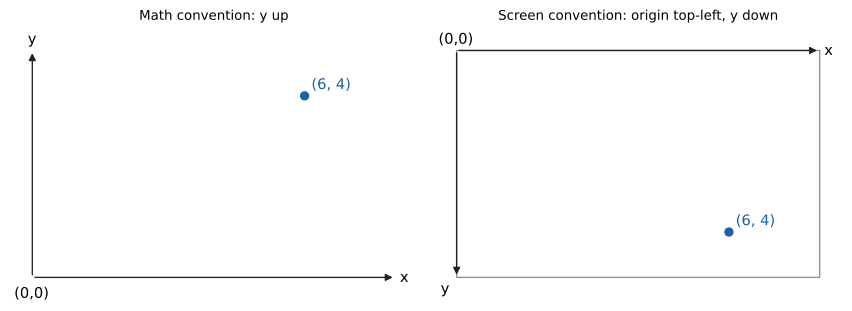
Displays are scanned like text: left to right, top to bottom. So almost every screen, image format and windowing system puts the origin at the top-left corner, with \(x\) increasing to the right and \(y\) increasing downward. Pixel coordinates are also integers, and they number cells, not points: pixel \((0, 0)\) is the little square in the corner.
|
Screen coordinates and pixels
Screen (or device, pixel) coordinates place the origin at the top-left, with \(x\) (column) rightward and \(y\) (row) downward. A pixel ("picture element") is one cell of the grid. World coordinates are the mathematical coordinates of the scene being drawn. A viewport transform converts world to screen coordinates. |
10.11.3. The method: world to screen
To draw a mathematical scene centred on \((c_x, c_y)\) at \(s\) pixels per unit in a canvas \(W\) pixels wide and \(H\) high, combine three transformations from Section 10.9: translate the world centre to the origin, dilate by \(s\) (and reflect in the x-axis to flip \(y\)), then translate the origin to the canvas centre: Try it: Try the world-to-screen map.
The single minus sign in the row formula is the whole difference between "math" and "screen".
def world_to_screen(x, y, width, height, scale, cx=0.0, cy=0.0):
    """Map math coords (y up, centred on (cx, cy)) to pixel coords (y down)."""
    col = width / 2 + (x - cx) * scale
    row = height / 2 - (y - cy) * scale        # the minus sign flips y
    return round(col), round(row)

print(world_to_screen(0, 0, 800, 600, 50))
print(world_to_screen(3, 2, 800, 600, 50))
print(world_to_screen(-8, -6, 800, 600, 50))
(400, 300) (550, 200) (0, 600)
The world point \((3, 2)\), up and right of centre, lands above the centre row 300, at row 200, as it should.
|
Flipped y flips everything that depends on orientation
In screen coordinates a line that rises on screen has a negative slope numerically; an anticlockwise rotation formula appears clockwise; the "left-hand side" test from a line’s sign flips; and polygon vertex order that was anticlockwise becomes clockwise (which can turn a shoelace area negative, or make a renderer cull the faces you wanted to see). Decide on one convention per layer of your code and convert exactly once, at the boundary. |
10.12. Drawing a line on a pixel grid: Bresenham’s algorithm
10.12.1. The problem
A line on paper is infinitely thin and continuous. A screen can only light whole pixels. Given two pixel endpoints, which pixels should be lit so the result looks like a straight line — no gaps, no clumps — and can we do it fast, ideally using only integer addition?
10.12.2. Intuition
Consider a line whose slope is between 0 and 1 (gently rising, more across than up), from \((x_0, y_0)\) to \((x_1, y_1)\) with integer endpoints. Because it is flat-ish, we want exactly one pixel per column. Moving one column to the right, the line rises by \(m < 1\), so the next pixel is either straight across, \((x+1, y)\), or diagonally up, \((x+1, y+1)\). Choose whichever is closer to the true line. The tie-breaker is the midpoint between the two candidates, \((x+1, y+\tfrac12)\): if the true line passes above it, go up; otherwise go across.
The naive way computes \(y = y_0 + m(x - x_0)\) for each column and rounds. It works, but it uses floating point and a multiplication per pixel — expensive on 1960s plotters (where Jack Bresenham invented the method, at IBM in 1962) and still wasteful today. Bresenham’s insight is to track the sign of an integer error term that changes by a fixed amount each step.
10.12.3. Why it works
Let \(\Delta x = x_1 - x_0 > 0\) and \(\Delta y = y_1 - y_0\), with \(0 \le \Delta y \le \Delta x\). Write the line in the standard form of Section 10.5, scaled to integers:
\(F = 0\) on the line; \(F > 0\) for points below it (smaller \(y\) makes \(-\Delta x\,(y - y_0)\) larger). Evaluate at the midpoint and double to clear the \(\tfrac12\): define the decision variable \(D = 2F(x + 1, y + \tfrac12)\).
-
If \(D > 0\), the midpoint is below the line, so the line is closer to the upper pixel: choose \((x+1, y+1)\).
-
Otherwise choose \((x+1, y)\).
How does \(D\) change from one column to the next? \(F\) is linear, so moving one unit in \(x\) adds \(\Delta y\) to \(F\) (that is, \(2\Delta y\) to \(D\)), and moving one unit up in \(y\) subtracts \(\Delta x\) (\(2\Delta x\) from \(D\)). At the start, \(F(x_0, y_0) = 0\), so
Only integer additions and comparisons. No multiplication inside the loop, no rounding, no floating point.
Input: integer endpoints \((x_0, y_0)\), \((x_1, y_1)\) with \(x_0 < x_1\) and \(0 \le y_1 - y_0 \le x_1 - x_0\) (slope between 0 and 1).
Steps:
-
Set \(\Delta x = x_1 - x_0\), \(\Delta y = y_1 - y_0\), \(D = 2\Delta y - \Delta x\), \(y = y_0\).
-
For each \(x\) from \(x_0\) to \(x_1\) inclusive:
-
Plot pixel \((x, y)\).
-
If \(D > 0\): increase \(y\) by 1 and subtract \(2\Delta x\) from \(D\).
-
Add \(2\Delta y\) to \(D\).
-
Output: the list of pixels, one per column, each within half a pixel of the true line.
Other directions: for steep lines (slope > 1) swap the roles of \(x\) and \(y\); for leftward or downward lines step by \(-1\) instead of \(+1\). The general version below handles all eight octants at once.
10.12.4. Worked example
Draw the segment from \((1, 1)\) to \((8, 4)\). Here \(\Delta x = 7\), \(\Delta y = 3\), so \(2\Delta y = 6\), \(2\Delta x = 14\), and \(D_{\text{start}} = 6 - 7 = -1\). Try it: Step through this example.
| \(x\) | plot \(y\) | \(D\) on arrival | decision | true \(y\) at this \(x\) |
|---|---|---|---|---|
1 |
1 |
−1 |
\(D \le 0\): across; \(D = -1 + 6 = 5\) |
1.000 |
2 |
1 |
5 |
\(D > 0\): up; \(D = 5 - 14 + 6 = -3\) |
1.429 |
3 |
2 |
−3 |
across; \(D = 3\) |
1.857 |
4 |
2 |
3 |
up; \(D = 3 - 14 + 6 = -5\) |
2.286 |
5 |
3 |
−5 |
across; \(D = 1\) |
2.714 |
6 |
3 |
1 |
up; \(D = 1 - 14 + 6 = -7\) |
3.143 |
7 |
4 |
−7 |
across; \(D = -1\) |
3.571 |
8 |
4 |
−1 |
(endpoint) |
4.000 |
Pixels: \((1,1), (2,1), (3,2), (4,2), (5,3), (6,3), (7,4), (8,4)\). Compare each plotted \(y\) with the true \(y\) in the last column: every one is the nearest integer. (At \(x = 2\), for example, the true height is 1.429, closer to 1 than to 2, and the algorithm plotted 1.)
def bresenham_octant1(x0, y0, x1, y1):
    """Pixels for a line with x0 < x1 and 0 <= slope <= 1."""
    dx, dy = x1 - x0, y1 - y0
    D = 2 * dy - dx                    # decision variable
    y = y0
    pixels = []
    for x in range(x0, x1 + 1):
        pixels.append((x, y))
        if D > 0:                      # true line is above the midpoint
            y += 1
            D -= 2 * dx
        D += 2 * dy
    return pixels

print(bresenham_octant1(1, 1, 8, 4))
[(1, 1), (2, 1), (3, 2), (4, 2), (5, 3), (6, 3), (7, 4), (8, 4)]
The production version handles every direction with one loop by keeping signed step directions \(s_x, s_y\) and a combined error term: Try it: Run the all-octant version.
def bresenham(x0, y0, x1, y1):
    """Integer pixels on the segment (x0, y0)-(x1, y1); all octants."""
    pixels = []
    dx = abs(x1 - x0)
    dy = -abs(y1 - y0)                 # stored negative: simplifies the tests
    sx = 1 if x0 < x1 else -1          # step direction in x
    sy = 1 if y0 < y1 else -1          # step direction in y
    err = dx + dy                      # error term, scaled by 2 below
    while True:
        pixels.append((x0, y0))
        if x0 == x1 and y0 == y1:
            return pixels
        e2 = 2 * err
        if e2 >= dy:                   # time to step in x
            err += dy
            x0 += sx
        if e2 <= dx:                   # time to step in y
            err += dx
            y0 += sy

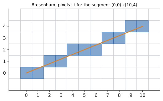
print(bresenham(0, 0, 10, 4))
print(bresenham(0, 0, 2, 5))
print(bresenham(3, 3, -2, 1))
[(0, 0), (1, 0), (2, 1), (3, 1), (4, 2), (5, 2), (6, 2), (7, 3), (8, 3), (9, 4), (10, 4)] [(0, 0), (0, 1), (1, 2), (1, 3), (2, 4), (2, 5)] [(3, 3), (2, 3), (1, 2), (0, 2), (-1, 1), (-2, 1)]
10.12.5. Alternatives and choosing
-
DDA (digital differential analyser): step \(x\) by 1 and add the floating-point slope \(m\) to \(y\) each step, rounding to plot. Simpler to explain; uses floating point; accumulated rounding error can drift on very long lines.
-
Bresenham / midpoint: integer-only and exact. The classic choice for aliased (hard-edged) lines, and the same midpoint idea draws circles (the midpoint circle algorithm) using the circle equation’s sign instead of the line’s.
-
Anti-aliased lines (Xiaolin Wu’s algorithm): light two pixels per column with brightness proportional to closeness. Smoother-looking; use when visual quality matters more than crispness.
Today GPUs rasterise lines and triangles in hardware, but the decision-variable idea — evaluate a linear function’s sign incrementally — is exactly how triangle rasterisers decide which pixels a triangle covers.
|
Ties are a choice, not a bug
When the true line passes exactly through a midpoint (\(D = 0\)), both candidate pixels are equally good. Different implementations break the tie differently: for the segment \((0, 0) \to (4, 2)\), the first-octant version above plots \((1, 0)\) and \((3, 1)\), while the all-octant version plots \((1, 1)\) and \((3, 2)\). Both are valid. But drawing \(A \to B\) and \(B \to A\) may then light slightly different pixels — which matters if you later erase a line by redrawing it. |
Try it: See the tie case.
|
Pixel-by-pixel
Click two pixels on a zoomed-in grid. Step through Bresenham one column at a time, watching the midpoint dot, the true line, and the value of \(D\) in a side panel. Toggle to DDA and to anti-aliased mode and compare the results on near-horizontal, 45°, and steep lines. Try it: Open the pixel-by-pixel lab |
10.13. Bounding boxes, point-in-circle tests, and distance metrics
10.13.1. The problem
A game has 500 moving objects. Checking whether every pair of detailed outlines overlaps is far too slow (\(500 \times 499 / 2 \approx 125{,}000\) pairs per frame, each expensive). How can coordinate geometry give cheap tests that rule out most pairs immediately?
10.13.2. Axis-aligned bounding boxes
Wrap each object in the smallest rectangle with sides parallel to the axes that contains it: its axis-aligned bounding box (AABB), described by \((x_{\min}, y_{\min}, x_{\max}, y_{\max})\) — the minimum and maximum of its vertices' coordinates. Two such boxes overlap exactly when their x-intervals overlap and their y-intervals overlap. Two intervals \(\lbrack a_1, a_2]\) and \(\lbrack b_1, b_2]\) overlap when each starts before the other ends: \(a_1 \le b_2\) and \(b_1 \le a_2\).
If the boxes do not overlap, the objects certainly do not; only if they do is the expensive exact test needed. This "cheap test first" pattern is called a broad phase followed by a narrow phase.
10.13.3. Point in circle, circle against circle
A point \((x, y)\) is inside or on the circle with centre \((h, k)\) and radius \(r\) when \((x - h)^2 + (y - k)^2 \le r^2\) — the circle equation from Section 10.7, turned into an inequality, with no square root. Two circles overlap when the distance between centres is at most the sum of the radii: \((h_1 - h_2)^2 + (k_1 - k_2)^2 \le (r_1 + r_2)^2\).
def bounding_box(points):
    xs = [x for x, _ in points]
    ys = [y for _, y in points]
    return min(xs), min(ys), max(xs), max(ys)   # (xmin, ymin, xmax, ymax)

def boxes_overlap(a, b):
    """Axis-aligned boxes (xmin, ymin, xmax, ymax); touching counts."""
    return a[0] <= b[2] and b[0] <= a[2] and a[1] <= b[3] and b[1] <= a[3]

def in_circle(p, centre, r):
    dx, dy = p[0] - centre[0], p[1] - centre[1]
    return dx*dx + dy*dy <= r*r                # no square root needed

ship = bounding_box([(2, 1), (6, 3), (4, 5)])
rock = bounding_box([(5, 4), (8, 6), (7, 9)])
print(ship, rock, boxes_overlap(ship, rock))
print(in_circle((5, 6), (2, 2), 5), in_circle((6, 6), (2, 2), 5))
(2, 1, 6, 5) (5, 4, 8, 9) True True False
The ship’s box spans \(x \in [2, 6]\), \(y \in [1, 5]\); the rock’s spans \(x \in [5, 8]\), \(y \in [4, 9]\). Both interval pairs overlap, so a narrow-phase test is needed. The point \((5, 6)\) is at squared distance \(9 + 16 = 25\) from \((2, 2)\): exactly on the radius-5 circle, so it counts as inside. The point \((6, 6)\) is at \(16 + 16 = 32 > 25\): outside.
|
A box test can say "maybe" but never a false "no"
Overlapping bounding boxes do not mean the objects touch: two thin diagonal sticks can have heavily overlapping boxes while being far apart. AABBs give false positives, never false negatives, which is exactly why they are only a first filter. Also decide deliberately whether touching edges count (\(\le\)) or not (\(<\)); mixing the two between functions causes flickering "is it colliding?" bugs. |
10.13.4. Euclidean versus Manhattan distance
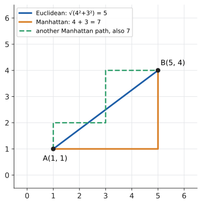
In Manhattan, a taxi cannot drive diagonally through buildings: it moves along streets in a grid. From \(A(1, 1)\) to \(B(5, 4)\) it must cover 4 blocks east and 3 blocks north, 7 blocks in total, whatever route it takes. The straight-line (Euclidean) distance is \(\sqrt{4^2 + 3^2} = 5\). Try it: Euclidean versus Manhattan distance.
|
Distance metrics
For points \(p = (x_1, y_1)\) and \(q = (x_2, y_2)\):
A metric is any distance function that is never negative, is zero only from a point to itself, is symmetric, and obeys the triangle inequality \(d(p, r) \le d(p, q) + d(q, r)\) (a detour never helps). All three above are metrics. |
def euclidean(p, q):
    return ((p[0] - q[0])**2 + (p[1] - q[1])**2) ** 0.5

def manhattan(p, q):
    return abs(p[0] - q[0]) + abs(p[1] - q[1])

def chebyshev(p, q):
    return max(abs(p[0] - q[0]), abs(p[1] - q[1]))

A, B = (1, 1), (5, 4)
print(euclidean(A, B), manhattan(A, B), chebyshev(A, B))
Try it: Drag A and B.
5.0 7 4
Always \(\text{Chebyshev} \le \text{Euclidean} \le \text{Manhattan}\): here \(4 \le 5 \le 7\).
Choosing a metric. Use Euclidean when movement is free in any direction (physics, drones, k-nearest-neighbours on continuous features). Use Manhattan when movement is restricted to a grid (city routing, 4-directional game maps, circuit-board wiring) or when you want a cheaper, absolute-value-only computation that is less dominated by one large difference. Use Chebyshev when diagonal moves cost the same as straight ones (8-directional grids, chess kings, some warehouse cranes that move both axes at once).
Try it: Watch Manhattan mislead A*.
|
Circles that are squares
A circle is "all points at distance \(r\) from a centre". Change the metric and the circle changes shape. In the Manhattan metric, the points at distance 1 from the origin satisfy \(|x| + |y| = 1\): a square standing on its corner (a diamond). In the Chebyshev metric, \(\max(|x|, |y|) = 1\) is an ordinary axis-aligned square. "Taxicab geometry" is a fully fledged non-Euclidean geometry in which many Euclidean theorems fail — for instance, two distinct points can have infinitely many midpoints. |
|
Unit circles in three metrics
Pick a metric (Euclidean, Manhattan, Chebyshev, or a general \(L^p\) with a slider for \(p\)) and the app draws every point at distance 1 from a centre you can drag. Watch the circle morph from diamond (\(p = 1\)) through round (\(p = 2\)) to square (\(p \to \infty\)). A second panel runs A* on a grid with each metric as heuristic and counts the nodes explored. |
10.13.5. Exercises
-
A canvas is 640 by 480 pixels, with world origin at the centre and 20 pixels per unit. Where is the world point \((-4, 3)\) drawn? Which world point is drawn at pixel \((100, 400)\)? Try it: Check your answer.
-
Use the first-octant Bresenham procedure to list the pixels from \((0, 0)\) to \((5, 2)\), showing \(D\) at each step. Try it: Check your answer.
-
Compute the Euclidean, Manhattan and Chebyshev distances between \((-2, 3)\) and \((4, -5)\).
-
Do the boxes \((0, 0, 4, 3)\) and \((5, 1, 7, 2)\) overlap? Do circles of radius 3 at \((0, 0)\) and radius 3.5 at \((4, 5)\) overlap?
-
A delivery robot moves in a warehouse along aisles parallel to the walls. Which metric should its route planner use as a heuristic, and why?
Answers
-
col \(= 320 + 20(-4) = 240\), row \(= 240 - 20(3) = 180\): pixel \((240, 180)\). Inverting, \(x = (\text{col} - 320)/20 = (100 - 320)/20 = -11\) and \(y = (240 - \text{row})/20 = (240 - 400)/20 = -8\): world point \((-11, -8)\).
-
\(\Delta x = 5\), \(\Delta y = 2\), \(D = 4 - 5 = -1\). x=0: plot (0,0), \(D \le 0\), \(D = -1 + 4 = 3\). x=1: plot (1,0), \(D > 0\), \(y = 1\), \(D = 3 - 10 + 4 = -3\). x=2: plot (2,1), \(D = 1\). x=3: plot (3,1), \(D > 0\), \(y = 2\), \(D = 1 - 10 + 4 = -5\). x=4: plot (4,2), \(D = -1\). x=5: plot (5,2). Pixels: \((0,0), (1,0), (2,1), (3,1), (4,2), (5,2)\).
-
\(|\Delta x| = 6\), \(|\Delta y| = 8\). Euclidean \(\sqrt{36 + 64} = 10\); Manhattan \(14\); Chebyshev \(8\).
-
Boxes: the x-intervals \(\lbrack 0, 4]\) and \(\lbrack 5, 7]\) do not overlap (\(5 > 4\)), so no. Circles: squared centre distance \(16 + 25 = 41\); \((3 + 3.5)^2 = 42.25\); \(41 \le 42.25\), so they overlap (just).
-
Manhattan: the robot can only move parallel to the axes, so the Manhattan distance is the true length of an unobstructed route and never overestimates the real path.
10.14. Interactive tools
Browser tools on the companion website that go with this chapter. Each example link in the chapter opens one of them with that example already set up.
10.15. Mastery check
-
Find the distance between \((-1, -3)\) and \((7, 3)\), and their midpoint.
-
Find, in slope-intercept and standard form, the line through \((2, -3)\) perpendicular to \(4x - 2y = 6\).
-
Find the centre and radius of \(x^2 + y^2 - 10x + 6y + 18 = 0\).
-
Identify the conic \(x^2 = -12y\) and give its focus and directrix.
-
The triangle \((0, 0), (2, 0), (0, 1)\) is rotated 90° anticlockwise about the origin and then translated by \((x, y) \mapsto (x + 3, y)\). Give the final vertices.
-
Find the distance between \((1, 1, 1)\) and \((3, -2, 7)\).
-
On an 800 by 600 canvas with the world origin at the centre and 50 pixels per unit, which pixel shows the world point \((2, -1)\)?
-
A taxi drives from block \((1, 2)\) to block \((6, -4)\) on a street grid. How far does it drive, and how far is that as the crow flies?
Decision rule: All correct without hesitation → move on to Chapter 11. Stuck on 1–2 → reread the relevant section (Section 10.3, Section 10.6, Section 10.7, Section 10.8, Section 10.9, Section 10.11) and redo its exercises. Stuck on more → work through all the section exercises first, and revisit Pythagoras in Chapter 9 and completing the square in Chapter 8.
Mastery check answers
-
\(\Delta x = 8\), \(\Delta y = 6\): \(d = \sqrt{64 + 36} = 10\). Midpoint \(\left(\frac{6}{2}, \frac{0}{2}\right) = (3, 0)\).
-
\(4x - 2y = 6 \Rightarrow y = 2x - 3\), slope 2. Perpendicular slope \(-\tfrac12\). \(y + 3 = -\tfrac12(x - 2) = -\tfrac12 x + 1\), so \(y = -\tfrac12 x - 2\). Standard form: multiply by 2, \(2y = -x - 4\), so \(x + 2y = -4\). Check \((2, -3)\): \(2 - 6 = -4\). Correct.
-
\((x^2 - 10x + 25) + (y^2 + 6y + 9) = -18 + 25 + 9 = 16\), so \((x - 5)^2 + (y + 3)^2 = 16\): centre \((5, -3)\), radius 4.
-
Parabola of the form \(x^2 = 4py\) with \(4p = -12\), \(p = -3\): opens downward, vertex at the origin, focus \((0, -3)\), directrix \(y = 3\).
-
Rotate with \((x, y) \mapsto (-y, x)\): \((0, 0), (0, 2), (-1, 0)\). Translate: \((3, 0), (3, 2), (2, 0)\).
-
Differences \(2, -3, 6\): \(\sqrt{4 + 9 + 36} = \sqrt{49} = 7\).
-
col \(= 400 + 50 \cdot 2 = 500\); row \(= 300 - 50 \cdot (-1) = 350\). Pixel \((500, 350)\).
-
Manhattan: \(|6 - 1| + |-4 - 2| = 5 + 6 = 11\) blocks. Euclidean: \(\sqrt{25 + 36} = \sqrt{61} \approx 7.81\) blocks.