Chapter 6. Systems of Equations

Volume 1: Foundations to Precalculus · Part II: Algebra

One equation with two unknowns has infinitely many solutions, so on its own it can’t pin anything down. Add a second, independent piece of information and the possibilities usually narrow to one. This chapter is about solving several equations at once. We start with pictures (lines that cross), work through the two classic hand methods (substitution and elimination), and then scale up to Gaussian elimination, the algorithm under every linear solver you’ll ever call. We finish with inequalities, feasible regions, and a first look at linear programming. Whenever several facts must hold at once (a phone fixing its position, a circuit simulator, a factory schedule, a model fitted to data) there is a system of equations underneath.

Where this chapter sits

You need: solving one linear equation and the line $y = mx + b$ (Chapter 5), and comfortable manipulation of expressions: expanding, collecting like terms, rearranging (Chapter 4). Fractions show up in the coefficients (Chapter 2).

This chapter unlocks: matrices and their inverses (Chapter 27), which recast everything here in a compact notation; fitting curves through points (Chapter 7); least-squares regression (Chapter 31); conditioning and floating-point stability (Chapter 32); and optimisation in general (Chapter 18, Chapter 20).

6.1. Why one equation is not enough

6.1.1. The problem

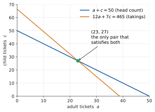
A school sells 50 tickets to a concert. Adult tickets cost $12 and child tickets cost $7. The till holds $465. How many of each were sold?

Call the number of adult tickets $a$ and the number of child tickets $c$. The money gives you one equation:

\[12a + 7c = 465.\]

That’s a perfectly good linear equation, but it can’t answer the question on its own. Plenty of pairs satisfy it if you ignore the head count: $a = 0, c = 66.43\ldots$ is one, $a = 38.75, c = 0$ is another, and there are infinitely many in between. The ticket count gives you a second fact:

\[a + c = 50.\]

Taken alone, this one is also satisfied by infinitely many pairs: (0, 50), (1, 49), (25, 25), and so on. But very few pairs satisfy both equations together. In fact exactly one does, and finding it is the subject of this chapter. (It’s $a = 23,\ c = 27$. Check it: $23 + 27 = 50$ and $12 \cdot 23 + 7 \cdot 27 = 276 + 189 = 465$.)

6.1.2. Intuition: each equation is a constraint

Think of each equation as a filter. Before any information arrives, every pair $(a, c)$ is possible. Each equation throws away everything that doesn’t satisfy it. With one equation in two unknowns you keep a whole line of candidates. A second equation keeps another line, and what survives both filters is where the two lines cross.

This gives a rule of thumb you’ll meet again and again:

To pin down $n$ unknowns you usually need $n$ independent equations.

"Usually" and "independent" are doing real work in that sentence. Two equations that say the same thing in different words ($a + c = 50$ and $2a + 2c = 100$) count as only one piece of information. Two equations that contradict each other can’t both hold, so nothing survives. We’ll be precise about both cases in Section 6.5.

System of equations

A system of equations is a collection of equations that must all hold at the same time, for the same values of the unknowns. A brace on the left is the usual way to show they belong together:

\[\begin{cases} a + c = 50 \\ 12a + 7c = 465 \end{cases}\]

British courses call these simultaneous equations, a name that stresses the "at the same time" part. US courses say systems of equations. They mean the same thing.

Solution of a system

A solution of a system is an assignment of values to all the unknowns that makes every equation true. For two unknowns $x, y$ a solution is an ordered pair $(x, y)$; for three it’s an ordered triple $(x, y, z)$. The solution set is the set of all solutions. It may contain exactly one element, none, or infinitely many.

Linear equation (in several variables)

An equation is linear if each unknown appears only to the first power, multiplied by a constant, and unknowns are never multiplied together. Its standard form is

\[a_1 x_1 + a_2 x_2 + \cdots + a_n x_n = b.\]

Here the subscripted $x_1, x_2, \ldots, x_n$ are the unknowns, the $a_i$ are their coefficients, and $b$ is the constant term (or right-hand side). So $3x - 2y = 7$ is linear. $xy = 7$, $x^2 + y = 1$ and $\sqrt{x} = y$ are not.

Two lines a+c=50 and 12a+7c=465 crossing at (23,27)

Figure 39. The ticket problem as two lines. Each line holds every pair that satisfies one equation; only the crossing point satisfies both.

Nine chapters, two thousand years

Systems of linear equations are among the oldest problems in written mathematics. The Chinese text The Nine Chapters on the Mathematical Art (compiled around the 1st century CE) has a chapter called fangcheng ("rectangular arrays"). It solves systems of three or more equations by laying out the coefficients on a counting board in columns and subtracting multiples of one column from another. That is Gaussian elimination, about 1,700 years before Gauss. The board even had a way to represent negative numbers: red rods for positive, black for negative.

6.2. Pictures first: the graphical method

6.2.1. Why a picture works

From Chapter 5 you know that the solutions of one linear equation in $x$ and $y$ form a straight line in the plane. A point lies on the line exactly when its coordinates satisfy the equation. So a point that satisfies two equations must lie on both lines at once, which means it’s an intersection point.

Solving a system of two linear equations = finding where two lines meet.

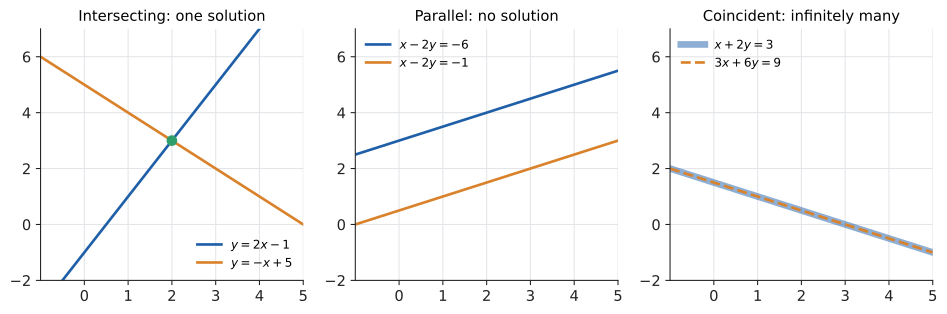
Two straight lines in a plane can relate in only three ways:

They cross at exactly one point, giving one solution.
They’re parallel (same slope, different intercept) and never meet, giving no solution.
They’re the same line drawn twice, so every point on it is shared, giving infinitely many solutions.

Nothing else can happen. Two distinct straight lines can’t meet at exactly two points. That fact matters: if you ever find two different solutions to a linear system, there must be infinitely many.

Three panels: intersecting lines, parallel lines, coincident lines

Figure 40. The three possible relationships between two lines, and the three possible sizes of the solution set.

Consistent, inconsistent, independent, dependent

A system is consistent if it has at least one solution, and inconsistent if it has none (parallel lines).
A consistent system is independent if the solution is unique (crossing lines), and dependent if there are infinitely many solutions (coincident lines). The second equation then "depends on" the first: it’s a multiple of it and adds no new information.

US textbooks use all four words. A common summary is "consistent independent / consistent dependent / inconsistent".

6.2.2. Worked example: solving by graphing

Solve

\[\begin{cases} y = 2x - 1 \\ y = -x + 5 \end{cases}\]

Both equations are already in slope–intercept form, $y = mx + b$.

First line. Slope $2$, intercept $-1$. Plot $(0, -1)$, then go 1 right and 2 up to $(1, 1)$, then again to $(2, 3)$.
Second line. Slope $-1$, intercept $5$. Plot $(0, 5)$, then 1 right and 1 down to $(1, 4)$, then $(2, 3)$.
Read off the crossing. Both lines pass through $(2, 3)$ (see the left panel of the figure above).
Check algebraically. First equation: $2(2) - 1 = 3$. Second: $-(2) + 5 = 3$. Both hold.

Solution: $(x, y) = (2, 3)$.

6.2.3. Predicting the case before you solve

Put both equations in slope–intercept form and compare:

Slopes	Intercepts	Result
different	anything	one solution (lines cross)
equal	different	no solution (parallel)
equal	equal	infinitely many (same line)

Slopes

Intercepts

Result

different

anything

one solution (lines cross)

equal

different

no solution (parallel)

equal

infinitely many (same line)

For example, $x - 2y = -6$ rearranges to $y = \tfrac12 x + 3$, and $x - 2y = -1$ to $y = \tfrac12 x + \tfrac12$. Same slope, different intercepts: parallel, so no solution. That’s the middle panel.

6.2.4. Failure modes of graphing

Graphs are approximate

Graphing is excellent for seeing what kind of answer to expect and terrible for precise answers. If the true solution is $(\tfrac{17}{11}, \tfrac{30}{11}) \approx (1.545, 2.727)$, no hand-drawn graph will tell you that. And when two lines are nearly parallel, a tiny drawing error moves the apparent crossing a long way (we’ll see in Section 6.11 that computers have a version of this problem too). Use graphs to sanity-check and to understand. Use algebra to get exact answers.

Graphing is still worth doing in three situations: when you want a quick estimate; when you need to understand what kind of answer exists before computing it; and when the equations aren’t linear and no algebraic method is convenient. Finding where $y = 2^x$ meets $y = x + 3$ is a graphing (or numerical) job, not a substitution job.

Drag the lines

Show two lines with sliders for each slope and intercept, and display the intersection point and its coordinates live. Rotate one line until it’s parallel to the other and watch the intersection run off to infinity and vanish. Then slide its intercept until the lines coincide. A second mode shows the equations in standard form $ax + by = c$ with sliders on $a, b, c$, so the learner sees how coefficients control slope.

Try it: Two lines with sliders

6.3. Substitution

6.3.1. The idea

If one equation tells you what one unknown equals in terms of the other, you can replace that unknown everywhere in the other equation. This is the "equals can be substituted for equals" principle from Chapter 4. What’s left is a single equation in a single unknown, which you already know how to solve (Chapter 5).

Why is this legitimate? Suppose $(x, y)$ is a solution of the system. Then $x$ really does equal $y + 2$ (say), so writing $y + 2$ wherever $x$ appeared changes nothing about whether the other equation is true. Every solution of the original system is also a solution of the reduced equation. Then, by back-substituting, every solution of the reduced equation gives back a solution of the system. Nothing is gained and nothing is lost.

Example 35. Procedure — Solving a 2×2 system by substitution

Input: two linear equations in unknowns $x$ and $y$.

Steps:

Choose an equation and an unknown that’s easy to isolate. Ideally pick one with coefficient $1$ or $-1$.
Rearrange that equation to make the chosen unknown the subject, e.g. $x = (\text{expression in } y)$.
Substitute that expression, in brackets, into the other equation.
Solve the resulting one-variable equation.
Substitute the value back into the rearranged equation from step 2 to get the other unknown.
Check the pair in both original equations.

Output: the solution $(x, y)$; or, if step 4 collapses to a false statement like $0 = 5$ or a true one like $0 = 0$, the conclusion "no solution" or "infinitely many" (see Section 6.5).

6.3.2. Worked example

Solve

\[\begin{cases} 3x + 2y = 16 & (1) \\ x - y = 2 & (2) \end{cases}\]

Equation (2) has $x$ with coefficient 1, so isolate $x$ there:

\[\begin{aligned} x - y &= 2 \\ x &= y + 2 && \text{(add } y \text{ to both sides)} \quad (3) \end{aligned}\]

Substitute (3) into (1), keeping the brackets:

\[\begin{aligned} 3(y + 2) + 2y &= 16 && \text{(replace } x \text{ by } y+2\text{)} \\ 3y + 6 + 2y &= 16 && \text{(distribute the 3)} \\ 5y + 6 &= 16 && \text{(collect like terms)} \\ 5y &= 10 && \text{(subtract 6)} \\ y &= 2 && \text{(divide by 5)} \end{aligned}\]

Back-substitute into (3): $x = 2 + 2 = 4$.

Check. (1): $3(4) + 2(2) = 12 + 4 = 16$. (2): $4 - 2 = 2$. Both hold, so $(x, y) = (4, 2)$.

6.3.3. The ticket problem by substitution

From $a + c = 50$ we get $c = 50 - a$. Substitute into $12a + 7c = 465$:

\[\begin{aligned} 12a + 7(50 - a) &= 465 \\ 12a + 350 - 7a &= 465 && \text{(distribute)} \\ 5a + 350 &= 465 && \text{(collect)} \\ 5a &= 115 \\ a &= 23 \end{aligned}\]

Then $c = 50 - 23 = 27$. That’s 23 adult tickets and 27 child tickets.

Three classic substitution slips

Dropping the brackets. Substituting $x = y + 2$ into $3x$ gives $3(y + 2) = 3y + 6$, not $3y + 2$. Always write the brackets first, then expand.
Substituting back into the same equation. If you rearranged (2) to get (3) and then substitute (3) into (2), you get $y + 2 - y = 2$, i.e. $2 = 2$. That’s true but tells you nothing, because you’ve used the same information twice. Substitute into the other equation.
Stopping at one unknown. The question asked for both. Finish with the back-substitution and the check.

Substitution shines when one equation already gives a variable explicitly ($y = \ldots$) or has a coefficient of $\pm 1$. It’s also the method of choice when one equation is not linear. For example, with $y = x^2$ and $y = x + 2$, substitution gives $x^2 = x + 2$, a quadratic you’ll learn to solve in Chapter 8. When every coefficient is something like 7 or 13, substitution drags fractions in early, and elimination is cleaner.

6.4. Elimination

6.4.1. The problem with substitution

Try substitution on

\[\begin{cases} 2x + 3y = 12 & (1) \\ 5x - 4y = 7 & (2) \end{cases}\]

Isolating anything gives fractions straight away: $x = 6 - \tfrac32 y$. It works, but it’s fiddly. Elimination avoids this.

6.4.2. Why adding equations is legal

If $A = B$ and $C = D$, then $A + C = B + D$: add equal things to equal things and the results are equal. Likewise, $kA = kB$ for any number $k$. So from any two equations in a system you can form a new true equation by scaling each one and adding them. The trick is to choose the scale factors so that one unknown cancels. Its coefficients become opposites and add to zero, which eliminates it.

There’s a subtle point: replacing one equation by "itself plus a multiple of the other" gives a new system with exactly the same solutions (as long as the multiplier on the equation being replaced is nonzero). The operation can be undone: just subtract the same multiple again. Reversible steps can’t create or destroy solutions. That one observation is the whole correctness argument for elimination, and later for Gaussian elimination.

Equivalent systems

Two systems are equivalent if they have exactly the same solution set. Elimination and substitution are chains of equivalent systems, each simpler than the one before, ending in a system so simple you can read the answer off (like $x = 3,\ y = 2$).

Example 36. Procedure — Solving a 2×2 system by elimination

Input: two linear equations in standard form $ax + by = c$, with like terms lined up in columns.

Steps:

Choose the unknown to eliminate. Prefer one whose coefficients are already equal or opposite, or have a small common multiple.
Multiply each equation by a nonzero number so that the chosen unknown has coefficients that are opposites (or equal). The least common multiple of the two coefficients keeps the numbers small.
Add the equations if the coefficients are opposites, or subtract if they’re equal. The chosen unknown disappears.
Solve the resulting one-variable equation.
Substitute the value into either original equation and solve for the other unknown.
Check in both original equations.

Output: the solution $(x, y)$, or the detection of "no solution" (a false statement such as $0 = -4$) or "infinitely many" ($0 = 0$).

6.4.3. Worked example

Solve $2x + 3y = 12$ (1) and $5x - 4y = 7$ (2).

Choose. The $y$-coefficients are $3$ and $-4$. They already have opposite signs, and their least common multiple is 12. So scale (1) by 4 and (2) by 3:

\[\begin{aligned} 4 \times (1):\quad 8x + 12y &= 48 \\ 3 \times (2):\quad 15x - 12y &= 21 \end{aligned}\]

Add (the $y$-terms are opposites):

\[\begin{aligned} (8x + 15x) + (12y - 12y) &= 48 + 21 \\ 23x &= 69 \\ x &= 3 && \text{(divide by 23)} \end{aligned}\]

Back-substitute into (1):

\[\begin{aligned} 2(3) + 3y &= 12 \\ 6 + 3y &= 12 \\ 3y &= 6 \\ y &= 2 \end{aligned}\]

Check in (2): $5(3) - 4(2) = 15 - 8 = 7$. The solution is $(x, y) = (3, 2)$.

Subtracting a negative

When you subtract one equation from another, the subtraction applies to every term, including the right-hand side and any terms that are already negative. From

\[\begin{aligned} 6x - 15y &= -72 \\ 6x + 8y &= 20 \end{aligned}\]

subtracting the second from the first gives $-15y - 8y = -72 - 20$, i.e. $-23y = -92$, so $y = 4$. A very common slip is to write $-15y + 8y$. If you find sign handling error-prone, multiply one equation by a negative number instead so you can always add. Adding is harder to get wrong.

6.4.4. Alternative approach: the general formula (Cramer’s rule)

Elimination is a procedure, so we can run it once on symbolic coefficients and get a formula that works for every 2×2 system. Take

\[\begin{cases} ax + by = c & (1) \\ dx + ey = f & (2) \end{cases}\]

To eliminate $y$, multiply (1) by $e$ and (2) by $b$, then subtract:

\[\begin{aligned} aex + bey &= ce && (e \times (1)) \\ bdx + bey &= bf && (b \times (2)) \\ (ae - bd)\,x &= ce - bf && \text{(subtract)} \end{aligned}\]

To eliminate $x$, multiply (1) by $d$ and (2) by $a$, then subtract the first from the second:

\[\begin{aligned} adx + bdy &= cd && (d \times (1)) \\ adx + aey &= af && (a \times (2)) \\ (ae - bd)\,y &= af - cd && \text{(subtract)} \end{aligned}\]

So, provided $ae - bd \neq 0$,

\[x = \frac{ce - bf}{ae - bd}, \qquad y = \frac{af - cd}{ae - bd}.\]

The quantity $ae - bd$ is called the determinant of the coefficient array. It’s zero exactly when the two lines have the same slope, that is, when there isn’t a unique solution. You’ll meet determinants properly in Chapter 27, where this formula becomes Cramer’s rule. Here it is as code:

def solve_2x2(a, b, c, d, e, f):
    """Solve  a*x + b*y = c,  d*x + e*y = f  by elimination."""
    det = a * e - b * d          # the "cross-multiplied" leftover coefficient
    if det == 0:
        raise ValueError("lines are parallel or coincident: no unique solution")
    x = (c * e - b * f) / det
    y = (a * f - c * d) / det
    return x, y

print(solve_2x2(2, 3, 12, 5, -4, 7))      # worked example
print(solve_2x2(1, 1, 50, 12, 7, 465))    # tickets
try:
    solve_2x2(2, 4, 6, 1, 2, 5)
except ValueError as err:
    print("error:", err)

(3.0, 2.0)
(23.0, 27.0)
error: lines are parallel or coincident: no unique solution

Should you memorise this formula? For 2×2 systems it’s handy, and it’s what you’d put in a tight inner loop (for example, intersecting two line segments in a game engine). But it doesn’t scale: the analogous formula for $n$ unknowns is hopelessly expensive. What scales is the procedure, which is why we come back to it in Section 6.9.

6.5. When the algebra says "never" or "always"

Graphs showed three possible outcomes. Here’s how each one looks when you do the algebra. You don’t need to graph anything: the algebra announces the case itself.

6.5.1. No solution: a contradiction appears

Solve

\[\begin{cases} 2x + 4y = 6 & (1) \\ x + 2y = 5 & (2) \end{cases}\]

Multiply (2) by 2 and subtract it from (1):

\[\begin{aligned} 2x + 4y &= 6 \\ 2x + 4y &= 10 && (2 \times (2)) \\ 0 &= -4 && \text{(subtract)} \end{aligned}\]

Both unknowns vanished and what’s left is false. That isn’t an arithmetic error. It’s the system telling you that no pair $(x, y)$ can satisfy both equations. Geometrically, $2x + 4y = 6$ and $x + 2y = 5$ are the parallel lines $y = -\tfrac12 x + \tfrac32$ and $y = -\tfrac12 x + \tfrac52$. The system is inconsistent, and the solution set is the empty set, written $\varnothing$.

The logic is a proof by contradiction (Chapter 22). If a solution existed, the derived equation $0 = -4$ would be true for it. Since $0 = -4$ is never true, no solution exists.

6.5.2. Infinitely many solutions: an identity appears

Solve

\[\begin{cases} x + 2y = 3 & (1) \\ 3x + 6y = 9 & (2) \end{cases}\]

Multiply (1) by 3 and subtract from (2):

\[\begin{aligned} 3x + 6y &= 9 \\ 3x + 6y &= 9 && (3 \times (1)) \\ 0 &= 0 && \text{(subtract)} \end{aligned}\]

Now both unknowns vanish and what’s left is always true. Equation (2) is just three times equation (1), so it carries no new information. You really have one equation in two unknowns, and every point on the line $x + 2y = 3$ is a solution. The system is consistent and dependent.

How do you write down infinitely many solutions? Let one unknown be free and express the other in terms of it. Introduce a parameter $t$ (any real number) and set $y = t$. Then $x = 3 - 2t$:

\[(x, y) = (3 - 2t,\ t), \qquad t \in \mathbb{R}.\]

Here $t \in \mathbb{R}$ reads "$t$ is an element of the real numbers", i.e. $t$ can be any real number. Every value of $t$ produces one solution: $t = 0$ gives $(3, 0)$, $t = 1$ gives $(1, 1)$, $t = -2$ gives $(7, -2)$. You can check each one in both equations.

Parameter, parametric solution

A parameter is a letter that stands for an arbitrary value you’re free to choose, as opposed to an unknown you’re trying to find (compare Chapter 4). A parametric solution such as $(3 - 2t,\ t)$ describes an infinite solution set by saying how every solution is built from the parameter. The unknown you set equal to the parameter is called a free variable.

6.5.3. A quick test without solving

For $ax + by = c$ and $dx + ey = f$, compare the ratios of the coefficients:

$\dfrac{a}{d} \neq \dfrac{b}{e}$ (equivalently $ae - bd \neq 0$): exactly one solution.
$\dfrac{a}{d} = \dfrac{b}{e} \neq \dfrac{c}{f}$: no solution.
$\dfrac{a}{d} = \dfrac{b}{e} = \dfrac{c}{f}$: infinitely many.

(If any of $d, e, f$ is zero, use the cross-multiplied form, e.g. $ae = bd$, to avoid dividing by zero.)

0 = 0 does not mean x = 0

Students sometimes see $0 = 0$ and write "$x = 0$", or see $0 = -4$ and assume they slipped somewhere and start again. Learn to read these as messages: $0 = 0$ means "the equations were redundant"; $0 = \text{nonzero}$ means "the equations contradict each other". Do re-check your arithmetic once, because an arithmetic error can produce either, but then believe the result.

Computer-science connection: degenerate cases are where code breaks

The parallel and coincident cases are exactly the ones naive geometry code forgets. A function that intersects two line segments by computing $(ce - bf)/(ae - bd)$ will divide by zero when the segments are parallel, and for nearly parallel segments it will return a point miles away. Robust computational-geometry libraries handle "determinant exactly zero" as a special case, and "determinant tiny" as a separate, suspicious case, often using exact or adaptive-precision arithmetic for the sign test. When you write if det == 0 with floating-point numbers, you’re nearly always writing a bug; compare against a tolerance scaled to the size of the inputs instead. We return to this in Chapter 32.

6.6. Choosing a method for two equations

All three methods give the same answer when they work. They differ in effort, in error-proneness, and in what they tell you.

Method	Choose it when	Avoid it when
Graphing	You want to see the situation, estimate, or check the number of solutions; equations aren’t linear and nothing else is easy	You need an exact answer, or the lines are nearly parallel
Substitution	A variable already has coefficient \(\pm 1\), or an equation is given as \(y = \ldots\); one equation is nonlinear	Every coefficient is "awkward" (fractions appear at once)
Elimination	Equations are in standard form \(ax + by = c\); coefficients are integers; you’ll scale up to 3+ unknowns	An equation is nonlinear (you can’t cancel \(x^2\) against \(x\))
Formula (\(\det\))	Coding a 2×2 solver; symbolic coefficients	Hand-working larger systems

Method

Choose it when

Avoid it when

Graphing

You want to see the situation, estimate, or check the number of solutions; equations aren’t linear and nothing else is easy

You need an exact answer, or the lines are nearly parallel

Substitution

A variable already has coefficient $\pm 1$, or an equation is given as $y = \ldots$; one equation is nonlinear

Every coefficient is "awkward" (fractions appear at once)

Elimination

Equations are in standard form $ax + by = c$; coefficients are integers; you’ll scale up to 3+ unknowns

An equation is nonlinear (you can’t cancel $x^2$ against $x$)

Formula ($\det$)

Coding a 2×2 solver; symbolic coefficients

Hand-working larger systems

A practical habit: before choosing, clear fractions and decimals by multiplying each equation by a suitable number (Chapter 5). The system

\[\begin{cases} \tfrac{x}{2} + \tfrac{y}{3} = 4 \\[2pt] 0.3x - 0.2y = 0 \end{cases}\]

becomes $3x + 2y = 24$ (times 6) and $3x - 2y = 0$ (times 10), and adding them gives $6x = 24$ at once.

Another habit: look for symmetry. With $3c + 2m = 14.5$ and $2c + 3m = 13$, adding gives $5c + 5m = 27.5$, so $c + m = 5.5$. Subtracting gives $c - m = 1.5$. Two trivial equations replace two awkward ones.

6.6.1. Where you’d use this

Whenever two facts constrain two unknowns, you have a 2×2 system.

Sport. A basketball team scores 52 points from 23 field goals, all 2-pointers or 3-pointers. With $x$ twos and $y$ threes: $x + y = 23$ and $2x + 3y = 52$. Subtract twice the first from the second: $y = 6$, so $x = 17$. Check: $34 + 18 = 52$.
Economics. A market settles where supply meets demand. If suppliers offer quantity $q$ at price $p = 2 + 0.5q$ and buyers demand it at $p = 20 - q$, then $2 + 0.5q = 20 - q$ gives $q = 12$ and $p = 8$: the equilibrium is the crossing point of two lines.
Positioning. Your phone can locate itself from distances to known transmitters (GPS satellites, Wi-Fi access points). In a flat 2D version, beacons sit at $(0, 0)$, $(10, 0)$ and $(0, 10)$, and the measured squared distances are $25$, $65$ and $45$. Each distance gives a circle equation such as $x^2 + y^2 = 25$ and $(x - 10)^2 + y^2 = 65$. Subtracting the first from the second cancels $x^2$ and $y^2$, leaving the linear equation $-20x + 100 = 40$, so $x = 3$. The third beacon gives $-20y + 100 = 20$ in the same way, so $y = 4$. The position is $(3, 4)$. Real receivers do this in 3D with a fourth unknown (the clock error), and with more measurements than unknowns, solved by least squares (Section 6.11).

6.7. Exercises: two equations, two unknowns

(Recognition) Without solving, say whether each system has one solution, no solution, or infinitely many.
1. $y = 3x + 1$, $y = 3x - 4$
2. $2x - y = 4$, $6x - 3y = 12$
3. $x + y = 1$, $x - y = 1$
(Substitution) Solve $y = 4x - 3$, $2x + 3y = 19$.
(Elimination) Solve $3x + 4y = 10$, $2x - 5y = -24$.
(Fractions) Solve $\tfrac{x}{2} + \tfrac{y}{3} = 4$, $\tfrac{x}{4} - \tfrac{y}{6} = 0$.
(Word problem) Three coffees and two muffins cost $14.50. Two coffees and three muffins cost $13.00. Find the price of each.
(Parameter) For which value of $k$ does $kx + 2y = 5$, $3x + 6y = 1$ have no solution? Is there a value of $k$ that gives infinitely many?
(Modelling) A boat travels 24 km downstream in 2 hours and returns upstream in 3 hours. Find the boat’s speed in still water and the speed of the current.

Answers

(a) Same slope 3, different intercepts: no solution. (b) The second equation is 3 times the first: infinitely many. (c) Slopes $-1$ and $1$ differ: one solution, namely $(1, 0)$.
Substitute: $2x + 3(4x - 3) = 19 \Rightarrow 2x + 12x - 9 = 19 \Rightarrow 14x = 28 \Rightarrow x = 2$. Then $y = 4(2) - 3 = 5$. Check: $4 + 15 = 19$. Answer: $(2, 5)$.
Multiply the first by 2 and the second by 3: $6x + 8y = 20$, $6x - 15y = -72$. Subtract (first minus second): $23y = 92$, so $y = 4$. Then $3x + 16 = 10 \Rightarrow x = -2$. Check: $2(-2) - 5(4) = -24$. Answer: $(-2, 4)$.
Multiply the first by 6: $3x + 2y = 24$. Multiply the second by 12: $3x - 2y = 0$. Add: $6x = 24$, $x = 4$; then $2y = 3x = 12$, $y = 6$. Check: $2 + 2 = 4$ and $1 - 1 = 0$. Answer: $(4, 6)$.
$3c + 2m = 14.5$ and $2c + 3m = 13$. Add: $5c + 5m = 27.5 \Rightarrow c + m = 5.5$. Subtract: $c - m = 1.5$. Adding these: $2c = 7$, so $c = 3.50$ and $m = 2.00$. Coffee $3.50, muffin $2.00.
No solution needs $ae = bd$, i.e. $6k = 2 \cdot 3$, so $k = 1$. Then the equations are $x + 2y = 5$ and $x + 2y = \tfrac13$, which contradict each other, so there’s no solution. Infinitely many would need $\tfrac{k}{3} = \tfrac{2}{6} = \tfrac{5}{1}$, but $\tfrac26 \neq 5$, so no $k$ works.
Let $b$ be the boat speed and $c$ the current, both in km/h. Downstream speed is $24/2 = 12$, so $b + c = 12$. Upstream speed is $24/3 = 8$, so $b - c = 8$. Adding: $2b = 20$, $b = 10$, so $c = 2$. Boat 10 km/h, current 2 km/h.

US curriculum

Systems of two linear equations (graphing, substitution, elimination, and the "no solution / infinitely many" cases) are a core Algebra I topic, usually in grade 8 or 9. Common Core standards 8.EE.C.8 and A-REI.C.5–6 cover it. A-REI.C.5 explicitly asks students to justify why replacing an equation by itself plus a multiple of the other preserves the solutions, which is the argument in Section 6.4. The UK name "simultaneous equations" is unknown to most US students.

6.8. Three equations, three unknowns

6.8.1. The problem

A café sells three blends of coffee bean, and you want to know how many kilograms of each to roast. Or a physicist has three currents in a circuit. Or you want the parabola $y = ax^2 + bx + c$ through three given points (you’ll do this in the exercises). Three unknowns need three independent equations, and the methods above extend directly.

6.8.2. What it looks like

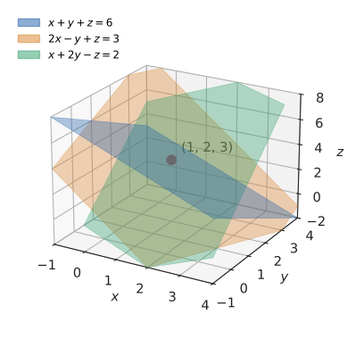
A linear equation in three unknowns, such as $x + y + z = 6$, describes a flat plane in three-dimensional space. Three planes can meet in a single point (the typical case, shown below), or along a whole line (like the pages of a book meeting at the spine), or coincide entirely, or have no point common to all three. That last case covers parallel planes, but also three planes that meet pairwise in three parallel lines, like the faces of a triangular prism. So the menu of outcomes is the same as before: one solution, none, or infinitely many.

Three translucent planes intersecting at the point (1,2,3)

Figure 41. Three planes meeting at a single point. The solution of the system below is where all three intersect.

6.8.3. The method: eliminate the same variable twice

The strategy reduces the problem to one you’ve already solved:

Use two different pairs of equations to eliminate the same unknown. That leaves two equations in two unknowns.
Solve that 2×2 system.
Back-substitute to find the third unknown.

6.8.4. Worked example

Solve

\[\begin{cases} x + y + z = 6 & (1) \\ 2x - y + z = 3 & (2) \\ x + 2y - z = 2 & (3) \end{cases}\]

Eliminate $x$ using (1) and (2). Subtract 2 × (1) from (2):

\[\begin{aligned} (2x - y + z) - 2(x + y + z) &= 3 - 2(6) \\ 2x - y + z - 2x - 2y - 2z &= 3 - 12 \\ -3y - z &= -9 && (4) \end{aligned}\]

Eliminate $x$ again, using (1) and (3). Subtract (1) from (3):

\[\begin{aligned} (x + 2y - z) - (x + y + z) &= 2 - 6 \\ y - 2z &= -4 && (5) \end{aligned}\]

Solve the 2×2 system (4), (5). Equation (5) has $y$ with coefficient 1, so either method works. Eliminate $y$ by adding 3 × (5) to (4):

\[\begin{aligned} (-3y - z) + 3(y - 2z) &= -9 + 3(-4) \\ -3y - z + 3y - 6z &= -9 - 12 \\ -7z &= -21 \\ z &= 3 \end{aligned}\]

Back-substitute. From (5): $y = -4 + 2z = -4 + 6 = 2$. From (1): $x = 6 - y - z = 6 - 2 - 3 = 1$.

Check in all three originals. (1): $1 + 2 + 3 = 6$. (2): $2 - 2 + 3 = 3$. (3): $1 + 4 - 3 = 2$. The solution is $(x, y, z) = (1, 2, 3)$.

Eliminating different variables

The most common mistake with three unknowns is eliminating $x$ from one pair and $y$ from another. You end up with two equations that each still contain two unknowns, but not the same two, and you’ve made no progress. Decide on the variable first, then eliminate that variable twice.

The second most common mistake is using the same pair twice, e.g. (1) & (2) and then (2) & (1) again. Every original equation must take part, or you’ve thrown away information.

Notice the shape of what we did. We kept (1) as it was, replaced (2) and (3) by equations without $x$, then replaced one of those by an equation without $y$. The final system

\[\begin{cases} x + y + z = 6 \\ \phantom{x+{}} y - 2z = -4 \\ \phantom{x+y{}} -7z = -21 \end{cases}\]

is a triangle: the last equation has one unknown, the one above it two, the one above that three. Solving a triangle from the bottom up is trivial. Making the triangle is the hard part. Turning this observation into an algorithm is the next section.

6.8.5. Where you’d use this

Fitting a model to measurements. A ball’s height is recorded as 2 m at $t = 0$, 12.1 m at $t = 1$ s and 12.4 m at $t = 2$ s. If $h = at^2 + bt + c$, each reading is one linear equation in $a, b, c$: $c = 2$, $a + b + c = 12.1$, $4a + 2b + c = 12.4$. With $c = 2$, these become $a + b = 10.1$ and $4a + 2b = 10.4$; subtract twice the first from the second to get $2a = -9.8$. So $a = -4.9$, $b = 15$: the data recover $h = 2 + 15t - 4.9t^2$, with $a = -\tfrac12 g$ for $g = 9.8\ \text{m/s}^2$. This is the thrown ball of Chapter 8.
Chemistry. Balancing a reaction is a linear system with one equation per element. For propane burning, $\mathrm{C_3H_8} + a\,\mathrm{O_2} \to b\,\mathrm{CO_2} + c\,\mathrm{H_2O}$: carbon gives $b = 3$, hydrogen $2c = 8$, oxygen $2a = 2b + c$. The system is already triangular: $b = 3$, $c = 4$, $a = 5$. Larger reactions give larger systems, and software balances them with exactly the elimination of the next section.
Colour. A screen colour is a mix of red, green and blue light, and converting to another colour space (for example, the device-independent XYZ space used in colour management) is three linear equations in three unknowns. Converting back means solving them.

6.9. Gaussian elimination: the algorithm

6.9.1. The problem

A structural-engineering model might have 10,000 unknowns, a circuit simulator a million, a weather model far more. Nobody juggles named equations like "(4)" and "(5)" at that scale. We need a procedure that’s mechanical, works for any number of unknowns, detects the no-solution and infinitely-many cases automatically, and can be coded in a few lines. That’s Gaussian elimination.

6.9.2. Notation: the augmented matrix

Notice that the letters $x, y, z$ did no work in the elimination. They only marked which column each coefficient lived in. So drop them and keep just the numbers in a rectangular array:

\[\begin{cases} x + y + z = 6 \\ 2x - y + z = 3 \\ x + 2y - z = 2 \end{cases} \quad\longleftrightarrow\quad \left[\begin{array}{rrr|r} 1 & 1 & 1 & 6 \\ 2 & -1 & 1 & 3 \\ 1 & 2 & -1 & 2 \end{array}\right]\]

Each row is one equation. Each of the first three columns holds the coefficients of one unknown, and the column after the vertical bar holds the right-hand sides.

Matrix, augmented matrix, row echelon form, pivot

A matrix is a rectangular array of numbers arranged in rows (horizontal) and columns (vertical). An $m \times n$ matrix has $m$ rows and $n$ columns. Matrices get a full chapter of their own in Chapter 27.
The coefficient matrix of a linear system holds just the coefficients. The augmented matrix has the right-hand-side column attached ("augmented") after a vertical bar.
A matrix is in row echelon form when every row’s first nonzero entry is to the right of the first nonzero entry of the row above, and any all-zero rows are at the bottom. It’s a staircase ("échelon" is French for a rung of a ladder).
The first nonzero entry in each row of an echelon form is a pivot. The pivot is the entry you use to clear the entries beneath it.

6.9.3. Why it works: the three row operations

Everything we did by hand used only these three moves, each of which turns the system into an equivalent one (same solutions) because each can be undone:

Swap two rows. (Reorder the equations. Undo: swap back.)
Scale a row by a nonzero number. (Undo: divide by it.)
Replace a row by itself plus a multiple of another row. (Undo: subtract the same multiple.)

Notation: $R_2 \leftarrow R_2 - 2R_1$ means "replace row 2 by row 2 minus twice row 1". The arrow $\leftarrow$ is deliberately the programmer’s assignment, not an equation.

6.9.4. Worked example in matrix form

Here is the same system again, in matrix form.

Step 1: clear column 1 below the pivot $1$ in row 1.

\[\left[\begin{array}{rrr|r} 1 & 1 & 1 & 6 \\ 2 & -1 & 1 & 3 \\ 1 & 2 & -1 & 2 \end{array}\right] \xrightarrow[\;R_3 \leftarrow R_3 - R_1\;]{R_2 \leftarrow R_2 - 2R_1} \left[\begin{array}{rrr|r} 1 & 1 & 1 & 6 \\ 0 & -3 & -1 & -9 \\ 0 & 1 & -2 & -4 \end{array}\right]\]

Row 2: $(2, -1, 1, 3) - 2(1, 1, 1, 6) = (0, -3, -1, -9)$. Row 3: $(1, 2, -1, 2) - (1, 1, 1, 6) = (0, 1, -2, -4)$.

Step 2: choose a pivot for column 2. We could use $-3$, but then we’d have to add $\tfrac13$ of row 2 to row 3, which brings in fractions. Swapping rows 2 and 3 gives a pivot of 1 instead:

\[\xrightarrow{R_2 \leftrightarrow R_3} \left[\begin{array}{rrr|r} 1 & 1 & 1 & 6 \\ 0 & 1 & -2 & -4 \\ 0 & -3 & -1 & -9 \end{array}\right]\]

Step 3: clear column 2 below the pivot.

\[\xrightarrow{R_3 \leftarrow R_3 + 3R_2} \left[\begin{array}{rrr|r} 1 & 1 & 1 & 6 \\ 0 & 1 & -2 & -4 \\ 0 & 0 & -7 & -21 \end{array}\right]\]

Row 3: $(0, -3, -1, -9) + 3(0, 1, -2, -4) = (0, 0, -7, -21)$. This is row echelon form.

Step 4: back substitution. Read the rows as equations, bottom up:

\[\begin{aligned} -7z &= -21 &&\Rightarrow\quad z = 3 \\ y - 2z &= -4 &&\Rightarrow\quad y = -4 + 2(3) = 2 \\ x + y + z &= 6 &&\Rightarrow\quad x = 6 - 2 - 3 = 1 \end{aligned}\]

The solution is $(1, 2, 3)$, as before. This is the same calculation as the hand method in Section 6.8. Only the bookkeeping is different.

6.9.5. Reading off the special cases

The echelon form tells you which of the three cases you’re in:

A row of the form $\left[\begin{array}{ccc|c} 0 & 0 & 0 & k\end{array}\right]$ with $k \neq 0$ says $0 = k$: inconsistent, no solution.
A row of all zeros, $\left[\begin{array}{ccc|c} 0 & 0 & 0 & 0\end{array}\right]$, says $0 = 0$: a redundant equation. If, after discarding such rows, there are fewer pivots than unknowns, the unknowns without a pivot are free variables and there are infinitely many solutions.
A pivot in every unknown’s column (and no contradiction): exactly one solution.

For a square system (as many equations as unknowns), that last case is the typical one, and in Chapter 27 you’ll see it’s the case where the coefficient matrix is invertible.

Example 37. Procedure — Gaussian elimination with back substitution

Input: an $n \times n$ system, written as the augmented matrix $\lbrack A \mid \mathbf{b}]$.

Steps:

For each column $j = 1, 2, \ldots, n$:
1. Pivot. Among rows $j$ to $n$, pick a row whose entry in column $j$ is nonzero. By hand, prefer a $\pm 1$ or a small integer. By computer, pick the one with the largest absolute value (partial pivoting). Swap it into row $j$. If every candidate is zero, the matrix is singular: stop and report "no unique solution".
2. Eliminate. For each row $i$ below $j$, compute the multiplier $m = a_{ij} / a_{jj}$ and do $R_i \leftarrow R_i - m R_j$. Column $j$ is now zero below the pivot.
Back-substitute. For $i = n, n-1, \ldots, 1$: $x_i = \big(b_i - \sum_{k > i} a_{ik} x_k\big) / a_{ii}$, using the already-found $x_k$.

Output: the solution vector $(x_1, \ldots, x_n)$, or a report that the system is singular. In that case, inspect the echelon form for a contradiction (no solution) or free variables (infinitely many).

The symbol $\sum_{k > i}$ in the back-substitution step is sigma notation. It means "add up the following term for every $k$ greater than $i$ (and up to $n$)". In code it’s a sum(…) over a range, as you’ll see below. Sequences and sums get full treatment in Chapter 14.

6.9.6. Implementation

def gaussian_solve(A, b):
    """Solve A x = b for square A by Gaussian elimination with partial pivoting.

    A is a list of n rows (each a list of n numbers); b is a list of n numbers.
    Returns the solution as a list. Raises ValueError if A is singular.
    """
    n = len(A)
    # Build the augmented matrix [A | b] as a fresh copy (don't mutate inputs).
    M = [list(map(float, row)) + [float(rhs)] for row, rhs in zip(A, b)]

    # Forward elimination: make zeros below each pivot.
    for col in range(n):
        # Partial pivoting: choose the row with the largest |entry| in this column.
        pivot_row = max(range(col, n), key=lambda r: abs(M[r][col]))
        if abs(M[pivot_row][col]) < 1e-12:
            raise ValueError("matrix is singular (no unique solution)")
        M[col], M[pivot_row] = M[pivot_row], M[col]
        for r in range(col + 1, n):
            factor = M[r][col] / M[col][col]
            for k in range(col, n + 1):
                M[r][k] -= factor * M[col][k]

    # Back substitution: solve from the last row upwards.
    x = [0.0] * n
    for i in range(n - 1, -1, -1):
        known = sum(M[i][k] * x[k] for k in range(i + 1, n))
        x[i] = (M[i][n] - known) / M[i][i]
    return x


A = [[1, 1, 1],
     [2, -1, 1],
     [1, 2, -1]]
b = [6, 3, 2]
print(gaussian_solve(A, b))

[1.0, 2.0000000000000004, 3.0000000000000004]

Notice the trailing …0004. Because the program pivots on the largest entry (2 in column 1, not 1), it divides by numbers like 2 and 3 along the way, and binary floating point can’t represent $\tfrac13$ exactly (Chapter 1). The answer is correct to about 16 significant digits, which is as good as float gets. Exact answers would need fractions.Fraction instead of float.

Why pivot on the largest entry?

Two failure modes motivate pivoting.

A zero pivot. The system $0x + y = 2,\ x + y = 3$ has the unique solution $(1, 2)$, but naive elimination that always uses row 1 as the pivot divides by zero at once. Swapping rows fixes it.
A tiny pivot. If the pivot is $10^{-20}$ instead of 0, there’s no crash, but the multiplier is $10^{20}$ and rounding errors get amplified enormously. The program will return a confidently wrong answer.

Choosing the largest available pivot keeps every multiplier at most 1 in size and controls this growth. Real libraries always pivot. You’ll see why in detail in Chapter 32.

Computer-science connection: the cost of elimination

Count the work. Clearing column $j$ touches about $(n - j)$ rows, each with about $(n - j)$ entries, so the forward phase costs roughly

\[\sum_{j=1}^{n} (n - j)^2 \approx \frac{n^3}{3}\]

multiply–add operations. Back substitution is only about $n^2/2$. So Gaussian elimination is $O(n^3)$: doubling the number of unknowns multiplies the work by eight. For $n = 1000$ that’s about $3 \times 10^8$ operations, a fraction of a second on a laptop. For $n = 10^6$ it would be $3 \times 10^{17}$, which is why huge systems that are mostly zeros (sparse systems: circuits, finite-element meshes, PageRank) use specialised sparse or iterative solvers instead.

Two further facts worth knowing. First, the forward phase depends only on $A$, not on $\mathbf{b}$. Libraries record the multipliers as an LU factorisation and reuse it to solve for many right-hand sides at $O(n^2)$ each. Second, the algorithm can be done in place in the matrix’s own memory, and its loops are the ones BLAS/LAPACK tune for cache behaviour. Every call to numpy.linalg.solve ends up in LAPACK’s gesv routine, which is exactly this: LU factorisation with partial pivoting.

Gauss and the lost planet

On 1 January 1801 the astronomer Giuseppe Piazzi spotted a new object, the dwarf planet Ceres. He followed it for about 40 days before it disappeared into the Sun’s glare. Astronomers expected it to be lost. The 24-year-old Carl Friedrich Gauss fitted an orbit to Piazzi’s handful of observations, and in December 1801 Ceres was found almost exactly where he predicted. Fitting the orbit required solving systems of linear equations, many more equations than unknowns, in the least-squares sense (previewed in Section 6.11), and the elimination procedure Gauss described for it is the one now named after him.

Watch the staircase form

Display a 3×3 or 4×4 augmented matrix with a "step" button. Each press performs one row operation and highlights the pivot, the row being changed, and the multiplier. Alongside, a 3D view shows the three planes; after each row operation the planes move but their common point stays fixed. That’s the geometric meaning of "equivalent system". Include a toggle between hand-friendly pivoting (smallest nonzero integer) and partial pivoting (largest absolute value), and a mode where the learner chooses each operation and the app checks it.

6.10. Exercises: three or more unknowns

(Application) Solve $x + y + z = 2$, $x - y + 2z = 9$, $2x + y - z = -3$.
(Recognition) Show that $x + y + z = 1$, $x + 2y + 3z = 2$, $2x + 3y + 4z = 4$ has no solution. What’s the quickest way to see it?
(Algorithm) Explain what happens if you run Gaussian elimination without row swaps on $y = 2$, $x + y = 3$ (written as $0x + 1y = 2$ first). What does gaussian_solve([[0, 1], [1, 1]], [2, 3]) return?
(Problem solving) Find the parabola $y = ax^2 + bx + c$ that passes through $(1, 2)$, $(2, 3)$ and $(3, 6)$.

Answers

Number the equations (1), (2), (3) in order. Eliminate $x$. (2) − (1): $-2y + z = 7$. (3) − 2(1): $-y - 3z = -7$. Eliminate $y$ from these two: twice the second is $-2y - 6z = -14$; subtract it from the first: $7z = 21$, so $z = 3$. Then $-y - 9 = -7$ gives $y = -2$, and $x = 2 - (-2) - 3 = 1$. Check: $1 + 2 + 6 = 9$ and $2 - 2 - 3 = -3$. Answer: $(1, -2, 3)$.
Add the first two equations: $2x + 3y + 4z = 3$. The third says $2x + 3y + 4z = 4$. The same left side can’t equal both 3 and 4. In matrix terms, $R_3 \leftarrow R_3 - R_1 - R_2$ produces $\left[\begin{array}{ccc|c}0&0&0&1\end{array}\right]$, i.e. $0 = 1$. Inconsistent. (The three planes meet pairwise in parallel lines.)
Naive elimination would compute the multiplier $1/0$ and crash (or produce inf/nan with NumPy floats). With partial pivoting, the code swaps the rows first, solves $x + y = 3,\ y = 2$, and returns [1.0, 2.0].
Substituting each point gives $a + b + c = 2$, $4a + 2b + c = 3$, $9a + 3b + c = 6$. Subtract consecutive equations to eliminate $c$: $3a + b = 1$ and $5a + b = 3$. Subtract these: $2a = 2$, so $a = 1$, $b = 1 - 3 = -2$, and $c = 2 - 1 + 2 = 3$. The parabola is $y = x^2 - 2x + 3$. Check $(3, 6)$: $9 - 6 + 3 = 6$. This is polynomial interpolation, which you’ll meet again in Chapter 7.

US curriculum

Three-variable systems usually appear in Algebra II (grade 10 or 11). Writing systems as matrices and solving them by row reduction (often to reduced row echelon form, "RREF", on a graphing calculator) appears in Algebra II or Precalculus. Common Core lists matrix methods as "+" (advanced) standards A-REI.C.8–9. Gaussian elimination as an algorithm, with pivoting and cost analysis, is a first-year university linear algebra or numerical methods topic.

6.11. Applications, and solving with a library

6.11.1. Mixtures

A lab needs 40 litres of a 45% acid solution, and it stocks 30% and 70% solutions. How much of each should it mix?

Let $x$ be the litres of 30% solution and $y$ the litres of 70%. There are two facts, giving two equations:

\[\begin{aligned} x + y &= 40 && \text{(total volume)} \\ 0.30x + 0.70y &= 0.45 \times 40 = 18 && \text{(litres of pure acid)} \end{aligned}\]

Substitute $y = 40 - x$:

\[\begin{aligned} 0.30x + 0.70(40 - x) &= 18 \\ 0.30x + 28 - 0.70x &= 18 \\ -0.40x &= -10 \\ x &= 25 \end{aligned}\]

So use 25 L of the 30% solution and 15 L of the 70% solution. Check: $7.5 + 10.5 = 18$ litres of acid. The same template, "one equation for the total amount, one for the total of some property", covers blending coffee beans, investing at two interest rates, and alloying metals.

6.11.2. Electrical circuits

Kirchhoff’s voltage law says that around any closed loop in a circuit, the voltage supplied equals the sum of the voltage drops across the resistors, where a resistor $R$ carrying current $I$ drops $RI$ volts (Ohm’s law). Take a circuit with two loops. Loop 1 has a 10 V battery and a 2 Ω resistor. Loop 2 has a 6 Ω resistor. A 3 Ω resistor sits on the wire the two loops share. Assign a loop current $I_1$ to loop 1 and $I_2$ to loop 2. The shared resistor carries $I_1 - I_2$:

\[\begin{aligned} \text{loop 1:}\quad 10 &= 2I_1 + 3(I_1 - I_2) &&\Rightarrow\quad 5I_1 - 3I_2 = 10 \\ \text{loop 2:}\quad 0 &= 3(I_2 - I_1) + 6I_2 &&\Rightarrow\quad -3I_1 + 9I_2 = 0 \end{aligned}\]

The second equation gives $I_1 = 3I_2$. Substituting into the first: $15I_2 - 3I_2 = 10$, so $I_2 = \tfrac{10}{12} = \tfrac56$ A, and $I_1 = \tfrac52 = 2.5$ A. Circuit simulators like SPICE do exactly this with thousands of loops or nodes, assembling one linear equation per loop or node and solving the resulting large sparse system.

6.11.3. Graphics: where do two lines cross?

In 2D graphics and games you constantly ask whether two moving things cross. Write a ray as a starting point plus a multiple of a direction. Ray 1 starts at $(0, 0)$ with direction $(4, 2)$, so its points are $(4t, 2t)$ for $t \ge 0$. Ray 2 starts at $(0, 3)$ with direction $(2, -1)$, so its points are $(2s, 3 - s)$. They meet where both coordinates agree:

\[\begin{cases} 4t = 2s \\ 2t = 3 - s \end{cases} \quad\Rightarrow\quad s = 2t,\quad 2t = 3 - 2t,\quad t = \tfrac34,\quad s = \tfrac32.\]

The crossing point is $(4 \cdot \tfrac34,\ 2 \cdot \tfrac34) = (3, 1.5)$. The parameter values carry extra information. If ray 2 were a segment that ends at $s = 1$, then $s = \tfrac32$ says the crossing lies beyond its end, so the segments don’t hit. In 3D the same idea (ray meets triangle) is a 3×3 system, and it’s the inner loop of ray tracing (Chapter 26).

6.11.4. Solving with NumPy

For real work you don’t hand-code elimination. You call a library:

import numpy as np

A = np.array([[1, 1, 1],
              [2, -1, 1],
              [1, 2, -1]], dtype=float)
b = np.array([6, 3, 2], dtype=float)
x = np.linalg.solve(A, b)
print(x)
print(np.allclose(A @ x, b))

# The two-loop circuit (mesh currents I1, I2 in amps)
C = np.array([[5, -3],
              [-3, 9]], dtype=float)
v = np.array([10, 0], dtype=float)
print(np.linalg.solve(C, v))

[1. 2. 3.]
True
[2.5        0.83333333]

Here A @ x is matrix–vector multiplication (Chapter 27). It recomputes every left-hand side, so np.allclose(A @ x, b) is the computer’s version of "check in all the original equations".

So why learn it by hand? Four reasons:

Setting up the system is the hard part, and no library does it for you. Choosing unknowns and translating each fact into an equation is the real skill, and you can only check it if you understand what a solution means.
Interpreting failure. np.linalg.solve raises LinAlgError: Singular matrix for the parallel and coincident cases. Without knowing what singular means geometrically, you can’t tell whether your model is missing an equation or contains two contradictory ones.
Recognising structure. Triangular, symmetric, banded, sparse: knowing how elimination works tells you when a specialised (and often thousands of times faster) solver applies.
Judging trustworthiness, which is the next topic.

6.11.5. A warning about nearly parallel lines

Consider Try it: Nudge b and watch x; Nudge the nearly parallel lines.

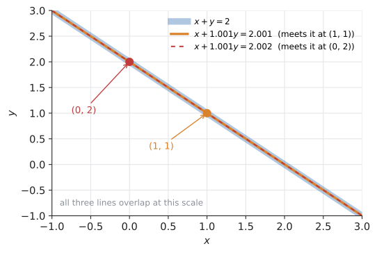
\[\begin{cases} x + y = 2 \\ x + 1.001y = 2.001 \end{cases} \qquad\text{versus}\qquad \begin{cases} x + y = 2 \\ x + 1.001y = 2.002 \end{cases}\]

The only difference is one right-hand side, changed by 0.001. Subtracting the first equation from the second gives $0.001y = 0.001$ in the first system and $0.001y = 0.002$ in the second. So the first system has solution $(1, 1)$ and the second has solution $(0, 2)$. A change of one part in two thousand in the data moved the answer by a full unit in each coordinate.

Nearly parallel lines whose intersection moves a long way when one line shifts slightly

Figure 42. Two nearly parallel lines. Nudging one line by 0.001 slides the intersection from (1, 1) to (0, 2).

import numpy as np

A = np.array([[1, 1],
              [1, 1.001]])
print(np.linalg.solve(A, [2, 2.001]))
print(np.linalg.solve(A, [2, 2.002]))   # right-hand side nudged by 0.001
print(round(np.linalg.cond(A)))

[1. 1.]
[0. 2.]
4002

The condition number (here about 4000) measures how much relative errors in the input can be amplified in the output. The library did nothing wrong: the problem itself is sensitive. If your inputs are measurements accurate to three digits, the answer to this system is essentially meaningless. Such a system is called ill-conditioned, and Chapter 32 explains how to measure and manage it. The geometric picture to keep in mind is two lines crossing at a shallow angle: the crossing point is poorly defined.

6.11.6. Regression preview: more equations than unknowns

Suppose you want the line $y = mx + b$ through the three data points $(0, 1)$, $(1, 3)$, $(2, 4)$. Each point gives one equation in the unknowns $m, b$:

\[\begin{cases} b = 1 \\ m + b = 3 \\ 2m + b = 4 \end{cases}\]

The first two give $b = 1, m = 2$, but then the third equation says $4 + 1 = 4$, which is false. Three equations in two unknowns is overdetermined, and real data almost never fits exactly. Instead you ask for the line that makes the total squared vertical error as small as possible: least squares. Minimising that error leads, as you’ll derive in Chapter 31, to a square 2×2 system called the normal equations:

\[\begin{cases} 3b + 3m = 8 \\ 3b + 5m = 11 \end{cases} \quad\Rightarrow\quad 2m = 3,\quad m = 1.5,\quad b = \tfrac{8 - 4.5}{3} = \tfrac76.\]

import numpy as np

xs = np.array([0, 1, 2], dtype=float)
ys = np.array([1, 3, 4], dtype=float)
A = np.column_stack([xs, np.ones_like(xs)])   # columns: x, 1  ->  unknowns m, b
(m, b), *_ = np.linalg.lstsq(A, ys, rcond=None)
print(round(m, 4), round(b, 4))

1.5 1.1667

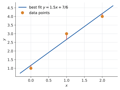
Three data points with a best-fit line and residual segments

Figure 43. No line passes through all three points; least squares picks the line that minimises the sum of squared vertical gaps (red).

So "fit a model to data", the foundation of statistics and machine learning, is at heart "solve a linear system", once the overdetermined system has been turned into a square one.

Computer-science connection: linear systems everywhere

Graphics: intersections (ray–plane, ray–triangle), solving for barycentric coordinates, and colour-space conversions are small linear systems solved millions of times per frame.
Simulation: physics engines solve linear systems for contact forces every frame. Implicit time-stepping methods for cloth and fluids solve huge sparse ones.
Machine learning: linear regression is a linear solve, and ridge regression adds one term to the diagonal. Newton-type optimisers solve a linear system at every step.
Search and ranking: PageRank is the solution of a very large linear system (equivalently, an eigenvector problem; see Chapter 28).
Networks: flows on networks (traffic, circuits, pipes) give one equation per node: "flow in = flow out".

In nearly all of these, the right question is not "can I solve it?" (the library can) but "is my system well-posed, well-conditioned, and structured enough to solve fast?"

US curriculum

Mixture, interest, and rate word problems with two unknowns are standard in Algebra I. Circuits appear in physics courses (AP Physics 1 and 2), usually solved by substitution. Linear regression on a calculator appears in Algebra I and AP Statistics, but the linear system behind it is normally left unexplained until college linear algebra.

6.12. Systems of linear inequalities and feasible regions

6.12.1. The problem

A small workshop makes tables and chairs. Each table earns $30 profit and each chair $20. The storeroom holds at most 40 items per week. Making a table takes 2 hours of labour and a chair 1 hour, and only 60 labour-hours are available. How many of each should it make to earn the most?

Let $x$ be the number of tables and $y$ the number of chairs. The constraints aren’t equations, because you don’t have to use all the storage or all the labour. They’re inequalities:

\[\begin{cases} x + y \le 40 & \text{(storage)} \\ 2x + y \le 60 & \text{(labour)} \\ x \ge 0,\ y \ge 0 & \text{(can't make negative furniture)} \end{cases}\]

The goal is to make $P = 30x + 20y$ as large as possible.

6.12.2. Intuition: half-planes

The equation $x + y = 40$ is a line. The inequality $x + y \le 40$ is that line together with everything on one side of it, which is called a half-plane. Which side? Test a point that’s not on the line. The origin is usually easiest: $0 + 0 \le 40$ is true, so the half-plane containing the origin is the one you want. (If the line passes through the origin, test a point like $(1, 0)$ instead.)

A system of inequalities asks for points satisfying all of them at once, which is the intersection of the half-planes. Graphically, shade each allowed region and look for where all the shadings overlap.

Half-plane, feasible region, vertex

A half-plane is the set of points on one side of a line. It’s closed (includes the boundary line, drawn solid) for $\le$ or $\ge$, and open (boundary excluded, drawn dashed) for $<$ or $>$.
The feasible region of a system of inequalities is the set of points satisfying every inequality. Points in it are feasible. If it’s empty, the system is infeasible.
A vertex (corner point) of the feasible region is a point where two boundary lines meet and every other constraint is satisfied. Finding each vertex means solving a 2×2 system of equations, which is where the earlier part of this chapter comes back in.

Example 38. Procedure — Graphing a system of linear inequalities

Input: linear inequalities in $x$ and $y$.

Steps:

For each inequality, draw its boundary line (replace the inequality sign by $=$). Draw it solid for $\le, \ge$ and dashed for $<, >$.
Test a point not on the line (usually $(0, 0)$). If it satisfies the inequality, that side is allowed; otherwise the other side is.
The feasible region is the overlap of all allowed sides.
Find each corner by solving the 2×2 system formed by the two boundary lines that meet there, then confirm the point satisfies every other inequality.

Output: the feasible region and its vertices (or the conclusion that it’s empty).

6.12.3. Worked example: the workshop

Boundaries. $x + y = 40$ passes through $(40, 0)$ and $(0, 40)$. $2x + y = 60$ passes through $(30, 0)$ and $(0, 60)$. Testing $(0, 0)$ in both inequalities gives $0 \le 40$ and $0 \le 60$, both true, so we want the side towards the origin each time. Together with $x, y \ge 0$, the feasible region is a four-sided polygon in the first quadrant. Try it: See the workshop region.

Vertices.

$(0, 0)$: where $x = 0$ meets $y = 0$.
$(30, 0)$: where $y = 0$ meets $2x + y = 60$. Check storage: $30 \le 40$. Feasible. (The other candidate on the $x$-axis, $(40, 0)$, fails labour: $80 > 60$.)
$(0, 40)$: where $x = 0$ meets $x + y = 40$. Check labour: $40 \le 60$. Feasible. (The candidate $(0, 60)$ fails storage.)
The crossing of the two resource lines. Subtract $x + y = 40$ from $2x + y = 60$ to get $x = 20$, so $y = 20$. That’s $(20, 20)$.

6.12.4. A taste of linear programming

Now the optimisation. For any target profit $P$, the points with $30x + 20y = P$ form a line with slope $-\tfrac32$. Different values of $P$ give parallel lines: level lines of the profit. Raising $P$ slides the line outward, away from the origin. The largest profit you can actually achieve corresponds to the last level line that still touches the feasible region as it slides outward, and because the region is a polygon with straight edges, that last contact happens at a corner.

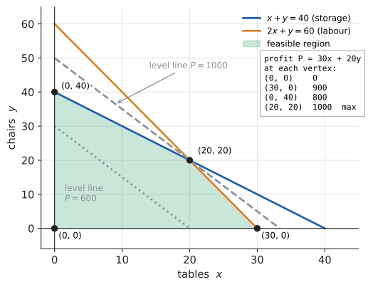
Feasible region bounded by x+y=40 and 2x+y=60 with vertices and profit level lines

Figure 44. The workshop’s feasible region (green), its four vertices with their profits, and two profit level lines. Pushing the level line outward, the last feasible point it touches is the vertex (20, 20).

So you only need to check the vertices:

Vertex \((x, y)\)	Profit \(P = 30x + 20y\)
\((0, 0)\)	\(0\)
\((30, 0)\)	\(900\)
\((20, 20)\)	\(600 + 400 = 1000\)
\((0, 40)\)	\(800\)

Vertex $(x, y)$

Profit $P = 30x + 20y$

$(0, 0)$

$0$

$(30, 0)$

$900$

$(20, 20)$

$600 + 400 = 1000$

$(0, 40)$

$800$

The best plan is 20 tables and 20 chairs, for $1,000 profit. It uses all the storage ($20 + 20 = 40$) and all the labour ($40 + 20 = 60$). Both constraints are binding.

Corner-point principle

A linear program (LP) maximises or minimises a linear objective function (like $30x + 20y$) subject to linear inequality constraints. The corner-point principle: if an LP has an optimal solution and its feasible region has at least one vertex, then some vertex is optimal. (If the objective’s level lines are parallel to an edge, every point on that edge ties.)

Here’s the "check every vertex" method as code. It generates every pair of boundary lines, solves each 2×2 system, keeps the feasible points, and picks the best:

from itertools import combinations

# Each constraint is (a, b, c) meaning a*x + b*y <= c.
constraints = [(1, 1, 40),    # storage
               (2, 1, 60),    # labour
               (-1, 0, 0),    # x >= 0  written as  -x <= 0
               (0, -1, 0)]    # y >= 0
profit = lambda x, y: 30 * x + 20 * y

best = None
for (a1, b1, c1), (a2, b2, c2) in combinations(constraints, 2):
    det = a1 * b2 - b1 * a2
    if det == 0:
        continue                          # parallel boundaries never meet
    x = (c1 * b2 - b1 * c2) / det + 0.0   # "+ 0.0" turns -0.0 into 0.0
    y = (a1 * c2 - c1 * a2) / det + 0.0
    if all(a * x + b * y <= c + 1e-9 for a, b, c in constraints):
        print(f"vertex ({x:g}, {y:g})  profit {profit(x, y):g}")
        if best is None or profit(x, y) > profit(*best):
            best = (x, y)
print("best:", best, profit(*best))

vertex (20, 20)  profit 1000
vertex (0, 40)  profit 800
vertex (30, 0)  profit 900
vertex (0, 0)  profit 0
best: (20.0, 20.0) 1000.0

6.12.5. Failure modes and limitations

When linear programming goes wrong

Unbounded regions. Drop the storage and labour limits and the profit can grow without limit. The LP has no optimum. Always check whether the feasible region is bounded in the direction you’re optimising.
Empty regions. Contradictory constraints ($x + y \le 10$ and $x + y \ge 20$) leave nothing feasible. That’s the inequality version of an inconsistent system.
Integer requirements. Our optimum $(20, 20)$ happened to be whole numbers. Often it isn’t (e.g. $(13.7, 22.4)$ tables and chairs), and rounding can break a constraint or miss the true best whole-number plan. Integer linear programming is a much harder problem (NP-hard in general).
Brute force doesn’t scale. With $m$ constraints in $n$ variables there can be up to $\binom{m}{n}$ candidate vertices: hundreds of billions for modest real problems. The vertex-enumeration code above is for understanding only.

Computer-science connection: linear programming and constraint satisfaction

Real LP solvers use the simplex method, which walks from vertex to adjacent vertex, always improving the objective, and stops when no neighbour is better. Each step is a Gaussian-elimination-style pivot, the same word used for the same operation. Alternatively they use interior-point methods, which cut through the middle of the region. LPs schedule airline crews, route network traffic (max-flow is an LP; see Chapter 25), allocate cloud resources, and balance diets and portfolios. Libraries such as SciPy’s linprog, Google OR-Tools, HiGHS and Gurobi do this at industrial scale.

More broadly, "find values satisfying all these constraints" is constraint satisfaction: type inference, package-version resolution (pip, npm, cargo), register allocation, and Sudoku are all examples. When the constraints are linear, the mathematics of this chapter gives you fast, exact tools. When they’re not, you get SAT and SMT solvers (Chapter 21).

War, breakfast, and a Nobel Prize

Linear programming was developed independently by Leonid Kantorovich in the Soviet Union (1939, for planning plywood production) and George Dantzig in the US (1947, for planning US Air Force logistics). "Programming" here meant planning or scheduling, as in a "programme" of activities, not writing code. One of the first test problems was George Stigler’s "diet problem": the cheapest combination of 77 foods meeting nine nutritional requirements. Kantorovich shared the 1975 Nobel Prize in economics for this work. Dantzig, famously, didn’t.

Slide the profit line

The learner enters up to five linear inequalities. The app shades the feasible region and labels its vertices. A draggable slider for $P$ moves the objective level line $30x + 20y = P$ across the plane, and the line turns red the moment it leaves the region. A second control rotates the objective (changing the profit ratio) so the learner can watch the optimal vertex jump from corner to corner, and see the tie when the objective lines up with an edge.

Try it: Slide the profit line

6.13. Exercises: inequalities and linear programming

(Recognition) Is the point $(3, 4)$ in the feasible region of $x + y \le 8$, $x - y \ge -2$, $y \ge 0$?
(Application) Maximise $P = 3x + 5y$ subject to $x + 2y \le 14$, $3x + 2y \le 18$, $x \ge 0$, $y \ge 0$. Try it: Check your answer.
(Problem solving) On the same region, minimise $C = x - y$. Then explain why maximising $P = x + y$ over the region $x \ge 0, y \ge 0, x - y \le 2$ has no answer.

Answers

$3 + 4 = 7 \le 8$ ✓; $3 - 4 = -1 \ge -2$ ✓; $4 \ge 0$ ✓. Yes, it’s feasible.
Vertices: $(0, 0)$; $(6, 0)$ (from $3x = 18$; check $6 \le 14$); $(0, 7)$ (from $2y = 14$; check $14 \le 18$); and the crossing of the two lines. Subtracting $x + 2y = 14$ from $3x + 2y = 18$ gives $2x = 4$, so $x = 2, y = 6$. Profits: $0, 18, 35, 6 + 30 = 36$. The maximum is $36$ at $(2, 6)$.
At the vertices, $C = 0, 6, -7, -4$. The minimum is $-7$ at $(0, 7)$. In the second region, the points $(t, t)$ for any $t \ge 0$ are feasible ($t - t = 0 \le 2$) with $P = 2t$, which grows without bound. The region is unbounded in the direction of increasing $P$, so no maximum exists.

US curriculum

Graphing linear inequalities in two variables and systems of them (Common Core A-REI.D.12) is part of Algebra I. Linear programming with the corner-point method appears in many Algebra II courses (and some Precalculus ones), usually as a word-problem unit. The simplex method and LP duality are college topics (operations research, algorithms courses).

6.14. Summary

A system asks for values that satisfy every equation at once. Geometrically, for two unknowns, it’s where lines cross. For three, it’s where planes meet.
There are always exactly three possibilities: one solution, no solution (the algebra produces $0 = \text{nonzero}$), or infinitely many (the algebra produces $0 = 0$; describe the solutions with a parameter).
Substitution is best when a variable is already isolated or easy to isolate, and when an equation is nonlinear. Elimination is best for standard-form linear equations, and it’s the version that scales.
Gaussian elimination is elimination as an algorithm: three reversible row operations turn the augmented matrix into a staircase, followed by back substitution. It costs $O(n^3)$, it needs pivoting to be reliable, and it’s what numpy.linalg.solve runs.
Libraries solve; you set up, interpret, and judge. Nearly parallel lines mean an ill-conditioned problem, where small input errors produce large output errors.
Systems of inequalities carve out feasible regions. A linear objective is optimised at a vertex, and vertices are 2×2 systems.

6.15. Interactive tools

Browser tools on the companion website that go with this chapter. Each example link in the chapter opens one of them with that example already set up.

6.16. Mastery check

Solve by any method: $y = 2x + 1$, $3x - y = 4$. Say why you chose that method.
Solve by elimination: $4x - 3y = 1$, $6x + 5y = 49$.
Classify $6x - 9y = 12$, $4x - 6y = 8$, and describe the full solution set.
Solve $x + 2y - z = 3$, $2x - y + z = 5$, $x + y + 2z = 10$.
How many litres each of a 10% and a 25% saline solution make 30 litres of 20% solution?
Maximise $4x + 3y$ subject to $x + y \le 10$, $x \le 6$, $y \le 8$, $x, y \ge 0$.
A colleague’s code calls np.linalg.solve on a 2×2 system and gets wildly different answers when the input data changes in the fourth decimal place. Give a geometric explanation, and say what single number you’d compute to confirm it.

Decision rule: All correct without hesitation → move on to Chapter 7 (or jump ahead to Chapter 27 if linear algebra is your priority). Stuck on 1–3 → reread Section 6.3, Section 6.4 and Section 6.5. Stuck on 4 → reread Section 6.8 and Section 6.9. Stuck on 5–7 → reread Section 6.11 and Section 6.12, then try the section exercises.

Try it: Check your answer.

Mastery check answers

Substitution, because the first equation already gives $y$. $3x - (2x + 1) = 4 \Rightarrow x - 1 = 4 \Rightarrow x = 5$, then $y = 11$. Check: $15 - 11 = 4$. Answer: $(5, 11)$.
Multiply the first by 3 and the second by 2 to match the $x$-coefficients: $12x - 9y = 3$ and $12x + 10y = 98$. Subtract the first from the second: $19y = 95$, so $y = 5$. Then $4x - 15 = 1 \Rightarrow x = 4$. Check: $24 + 25 = 49$. Answer: $(4, 5)$.
Divide the first by 3 and the second by 2: both become $2x - 3y = 4$. Same line, so the system is consistent and dependent, with infinitely many solutions. With parameter $t$ (so $y = t$): $(x, y) = \big(\tfrac{4 + 3t}{2},\ t\big)$, $t \in \mathbb{R}$. For example, $t = 0$ gives $(2, 0)$.
Number the equations (1), (2), (3). Add (1) and (2) to eliminate $z$: $3x + y = 8$. Take 2 × (2) minus (3): $(4x - 2y + 2z) - (x + y + 2z) = 10 - 10$, i.e. $3x - 3y = 0$, so $x = y$. Then $4x = 8$, so $x = 2$ and $y = 2$. From (2): $z = 5 - 4 + 2 = 3$. Check (1): $2 + 4 - 3 = 3$; (3): $2 + 2 + 6 = 10$. Answer: $(2, 2, 3)$.
$x + y = 30$ and $0.10x + 0.25y = 0.20 \times 30 = 6$. Substitute $x = 30 - y$: $3 - 0.10y + 0.25y = 6 \Rightarrow 0.15y = 3 \Rightarrow y = 20$, so $x = 10$. That’s 10 L of 10% and 20 L of 25%. Check: $1 + 5 = 6$.
Vertices: $(0,0)$, $(6,0)$, $(6,4)$ (from $x = 6$ and $x + y = 10$), $(2,8)$ (from $y = 8$ and $x + y = 10$), and $(0,8)$. Objective values: $0, 24, 36, 32, 24$. The maximum is $36$ at $(6, 4)$.
The two lines are nearly parallel, so they cross at a shallow angle, and a tiny shift in either line slides the crossing point a long way. The system is ill-conditioned. Compute the condition number, np.linalg.cond(A). A large value (say $10^3$ or more relative to the precision of the data) confirms it. The fix lies in the model (better data, a different formulation), not in a different solver. See Chapter 32.