Volume 1: Foundations to Precalculus · Part IV: Functions, Trigonometry, and Precalculus
Chapter 14. Sequences, Series, and Summation Notation
Chapter map: a sequence is an ordered list of numbers produced by a rule; a series is what you get when you add the terms up. This chapter teaches you to describe sequences two ways (explicitly and recursively), to read and write the compact notations Σ and Π, to sum arithmetic and geometric series in closed form, and to ask the deep question "does an infinite sum have a value?" Along the way you will meet the same mathematics hiding in nested loops, growable arrays, recursive algorithms, and memoisation.
Why this chapter matters: a mortgage payment, a pension projection, the level of a medicine in your blood after a week of daily doses, the number of matches in a league season and the running time of a nested loop are all sums of sequences. With two formulas (arithmetic and geometric) you can compute them in one line instead of a spreadsheet of a thousand rows, and you can tell in advance whether a process settles down or runs away.
14.1. Sequences: lists with a rule
14.1.1. The problem
You put $1{,}000 into an account paying 4% interest per year. What is the balance after 1 year, 2 years, 10 years? A ball is dropped from 10 m and each bounce reaches 60% of the previous height. How high is the seventh bounce? A theatre has 20 seats in the front row and each row behind has 2 more. How many seats are in row 30?
Each question asks for one item in an ordered list of numbers that is generated by a rule. That list is a sequence, and the questions become: given the rule, find the nth item — and, later, add the items up.
14.1.2. Intuition
Think of a sequence as an array that never ends, indexed by position: a[1], a[2], a[3], …. The interesting thing is never the individual numbers; it is the rule that produces them. Once you know the rule, you can answer questions about item 1,000,000 without writing out the first 999,999.
There are two natural ways to state a rule, and programmers already know both:
-
Explicit (closed-form): a formula that gives the nth term directly from n. Like a pure function
a(n). -
Recursive: a starting value plus a rule for getting each term from the previous one(s). Like a loop that updates a variable, or a recursive function.
|
Sequence, term, index
A sequence is an ordered list of numbers \(a_1, a_2, a_3, \ldots\). Each number is a term. The subscript is the index (position): \(a_n\) is read "a sub n" and means "the term in position n". The whole sequence is written \((a_n)\) or \(\{a_n\}_{n \ge 1}\). A sequence may be finite (it stops) or infinite (it goes on forever). Formally, an infinite sequence is just a function whose domain is the positive integers: \(a_n\) is another way of writing \(a(n)\). |
|
Explicit formula and recursive definition
An explicit formula (or closed form, or general term) gives \(a_n\) directly in terms of \(n\), for example \(a_n = n^2\). A recursive definition (or recurrence relation) gives one or more initial conditions and a rule expressing \(a_n\) in terms of earlier terms, for example \(a_1 = 1,\ a_n = a_{n-1} + 2n - 1\). Without the initial condition a recurrence does not pin down a single sequence. |
14.1.3. Why both descriptions matter
Here is the same sequence, the perfect squares, described both ways:
Check the recursive version: \(a_2 = 1 + 3 = 4\), \(a_3 = 4 + 5 = 9\), \(a_4 = 9 + 7 = 16\). Each square is the previous square plus the next odd number. The explicit form is better for jumping straight to \(a_{1000} = 1{,}000{,}000\); the recursive form often reflects how the quantity actually arises — the bank adds interest to last year’s balance, the ball’s bounce depends on the previous bounce. Much of this chapter is about converting a recursive description (which is easy to write down from a story) into an explicit one (which is easy to compute and reason about).
def squares_explicit(n):
    return n * n

def squares_recursive(n):
    a = 1                       # initial condition a_1 = 1
    for k in range(2, n + 1):   # apply a_k = a_{k-1} + (2k - 1)
        a = a + (2 * k - 1)
    return a

print([squares_explicit(n) for n in range(1, 8)])
print([squares_recursive(n) for n in range(1, 8)])
[1, 4, 9, 16, 25, 36, 49] [1, 4, 9, 16, 25, 36, 49]
14.1.4. Worked example: finding a rule from terms
Find an explicit formula for \(2, 5, 10, 17, 26, \ldots\).
Step 1 — look at differences. \(5-2=3,\ 10-5=5,\ 17-10=7,\ 26-17=9\). The differences are consecutive odd numbers, which is the signature of squares (as we just saw).
Step 2 — compare with \(n^2\). For \(n = 1,2,3,4,5\): \(n^2 = 1, 4, 9, 16, 25\). Each given term is exactly one more.
Step 3 — state and check. \(a_n = n^2 + 1\). Check \(n = 4\): \(16 + 1 = 17\). ✓
|
A few terms never determine a sequence
"What comes next: 1, 2, 4, 8, 16, …?" Most people say 32, and the rule \(a_n = 2^{n-1}\) agrees. But the number of regions formed by joining \(n\) points on a circle in general position goes 1, 2, 4, 8, 16, 31. Finitely many terms are consistent with infinitely many rules. In mathematics a sequence is defined by its rule, not by its first few terms; "spot the pattern" puzzles are guesses, not deductions. |
|
Indexing from 0 or 1
Mathematicians often start at \(a_1\); programmers (and many mathematicians when it is more natural) start at \(a_0\). Neither is wrong, but mixing them causes off-by-one errors exactly as in code. Always check which index the first term has before using a formula. In this chapter we say explicitly which we are using. |
14.2. Arithmetic and geometric sequences
Two families of sequences account for a remarkable fraction of real applications: those that grow by adding the same amount each step and those that grow by multiplying by the same amount each step.
14.2.1. The problem
The theatre (20 seats in row 1, two more each row) and the savings account (multiply by 1.04 each year) are the two prototypes. We want explicit formulas for both.
|
Arithmetic sequence
An arithmetic sequence (or arithmetic progression, AP) adds a fixed common difference \(d\) each step: \(a_n = a_{n-1} + d\). Its explicit form, with first term \(a_1\), is \(a_n = a_1 + (n-1)d.\) The word is pronounced a-rith-MET-ic (stress on the third syllable) when used as an adjective. |
|
Geometric sequence
A geometric sequence (or geometric progression, GP) multiplies by a fixed common ratio \(r\) each step: \(a_n = r\,a_{n-1}\). Its explicit form, with first term \(a_1\), is \(a_n = a_1 r^{\,n-1}.\) |
14.2.2. Why the formulas work
For an arithmetic sequence, getting from term 1 to term \(n\) takes \(n-1\) steps, each adding \(d\):
The "\(n-1\)" is the classic fence-post count: \(n\) posts, \(n-1\) gaps. For a geometric sequence the same unrolling multiplies instead of adds, giving \(a_n = a_1 r^{n-1}\).
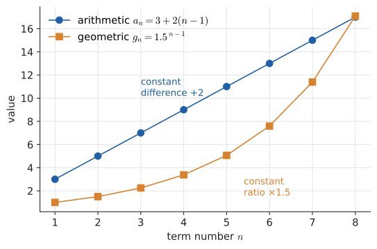
Seen as functions of \(n\), an arithmetic sequence is a linear function sampled at whole numbers (slope \(d\)), and a geometric sequence is an exponential function sampled at whole numbers (base \(r\)). The picture makes the difference unforgettable.
14.2.3. The method
Input: several consecutive terms of a sequence.
Steps:
-
Compute consecutive differences \(a_{k+1} - a_k\). If they are all equal to some \(d\), the sequence is arithmetic: \(a_n = a_1 + (n-1)d\).
-
Otherwise compute consecutive ratios \(a_{k+1}/a_k\) (all terms nonzero). If they are all equal to some \(r\), the sequence is geometric: \(a_n = a_1 r^{n-1}\).
-
If neither, try second differences (constant second differences mean a quadratic in \(n\)) or compare with known sequences.
-
Check the formula against a term you did not use to derive it.
Output: an explicit formula \(a_n\).
14.2.4. Worked examples
Theatre seats. \(a_1 = 20\), \(d = 2\). Row 30 has
Which term? In \(7, 11, 15, 19, \ldots\), is 203 a term, and if so which one? Here \(d = 4\), so \(a_n = 7 + 4(n-1) = 4n + 3\). Solve \(4n + 3 = 203\): \(4n = 200\), \(n = 50\). Yes, 203 is the 50th term. (If solving had given a non-integer \(n\), the number would not be in the sequence.)
Bouncing ball. The first bounce reaches 6 m (60% of 10 m), so \(a_1 = 6\), \(r = 0.6\). The seventh bounce reaches
How many years to double? At 4% per year, the balance after \(n\) years is \(1000 \cdot 1.04^{n}\) (indexing from \(n = 0\), the initial deposit). Doubling means \(1.04^{n} = 2\), so, taking logarithms (Chapter 12),
so the balance first exceeds $2,000 after 18 years.
|
Negative and fractional ratios
A geometric sequence can have \(r < 0\): \(3, -6, 12, -24, \ldots\) has \(r = -2\) and alternates in sign. With \(0 < |r| < 1\) the terms shrink towards zero (decay). With \(r = 1\) the sequence is constant; with \(r = 0\) it collapses to zero after the first term. Check the sign of \(r\) carefully: \((-2)^{n-1}\) and \(-2^{n-1}\) are different things. |
14.2.5. Where you’d use this
-
Everyday (arithmetic): a taxi charges $3.50 to start plus $2.20 per mile. The fare after \(n\) miles is the arithmetic sequence \(a_n = 3.50 + 2.20n\), so a 12-mile ride costs \(3.50 + 26.40 = \$29.90\). Any "fixed fee plus a rate" price works this way: phone plans, gym memberships, parking.
-
Music (geometric): on a piano each semitone raises the frequency by the same factor, \(2^{1/12} \approx 1.0595\), so twelve semitones double it (an octave). The notes form a geometric sequence. From A at 440 Hz, the C three semitones up is \(440 \times 2^{3/12} \approx 523.25\) Hz.
-
Science (geometric): carbon-14 halves every 5,730 years, so after \(n\) half-lives a fraction \(0.5^n\) remains. A bone with 12.5% of its original carbon-14 has been through 3 half-lives: it is about 17,000 years old.
-
Computing (geometric): when a network request fails, well-behaved clients retry with exponential backoff: wait 0.1 s, then 0.2 s, 0.4 s, and so on (\(a_k = 0.1 \times 2^{k-1}\)). The 8th retry waits \(0.1 \times 2^7 = 12.8\) s. Doubling the gap stops thousands of clients from hammering a struggling server in lock-step.
|
Arithmetic and geometric means
The middle term of three consecutive terms of an arithmetic sequence is the average of its neighbours, \(\tfrac{a+c}{2}\) — hence the arithmetic mean. In a geometric sequence the middle term is \(\sqrt{ac}\), the geometric mean. That is where the names come from. The geometric mean is the right average for growth rates: if an investment grows 50% one year and falls 50% the next, the average growth factor is \(\sqrt{1.5 \times 0.5} \approx 0.866\), not 1. |
14.3. Summation notation: Σ and Π
14.3.1. The problem
Before adding up sequences we need a way to write a sum of many terms without ellipses and ambiguity. "\(1 + 4 + 9 + \cdots + 100\)" relies on the reader guessing the pattern. Mathematics has a precise, compact notation for this — and it is exactly a for loop.
14.3.2. Reading Σ piece by piece
Here is the notation in full:
Read it as "the sum, for \(i\) from 1 to \(n\), of \(x\) sub \(i\)". Each piece has a job:
-
\(\Sigma\) — the capital Greek letter sigma, for "S" as in sum. It says: add things up.
-
\(i\) (below the sigma, before the equals sign) — the index of summation, a counter variable. It is a dummy variable: it exists only inside the sum, just as a loop variable exists only inside the loop. Writing \(k\) or \(j\) instead changes nothing.
-
\(1\) (below, after the equals sign) — the lower bound: the first value the index takes.
-
\(n\) (above) — the upper bound: the last value the index takes. Both bounds are inclusive.
-
\(x_i\) (to the right) — the summand, the expression evaluated for each value of the index and then added.
So \(\sum_{i=1}^{n} x_i\) means \(x_1 + x_2 + \cdots + x_n\). The index steps by 1 from lower bound to upper bound; there is no "step" parameter.
# Sigma notation is a for-loop
def sigma(lo, hi, term):
    total = 0
    for i in range(lo, hi + 1):   # inclusive upper bound, like the maths
        total += term(i)
    return total

print(sigma(1, 100, lambda i: i))          # 1 + 2 + ... + 100
print(sigma(1, 5, lambda k: k * k))        # 1 + 4 + 9 + 16 + 25
print(sum(k * k for k in range(1, 6)))     # the idiomatic one-liner
5050 55 55
Note the hi + 1: Python’s range excludes its end point, sigma includes it. That single fact causes most off-by-one errors when translating formulas into code.
|
Sigma notation
\(\displaystyle\sum_{i=m}^{n} f(i) = f(m) + f(m+1) + \cdots + f(n)\). The index \(i\) is a dummy variable; \(m\) and \(n\) are the lower and upper bounds (inclusive); \(f(i)\) is the summand. If \(n < m\) the sum is empty and equals 0. The number of terms is \(n - m + 1\). |
14.3.3. Worked examples: reading and writing sigma
Expand. \(\sum_{k=2}^{5} (2k - 1)\): the index runs over \(k = 2, 3, 4, 5\), giving \(3 + 5 + 7 + 9 = 24\).
Expand with an index that appears as an exponent. \(\sum_{j=0}^{4} 3^{j} = 3^0 + 3^1 + 3^2 + 3^3 + 3^4 = 1 + 3 + 9 + 27 + 81 = 121\).
Summand not depending on the index. \(\sum_{i=1}^{6} 5 = 5 + 5 + 5 + 5 + 5 + 5 = 30\). The summand is evaluated six times, even though it ignores \(i\).
Compress. Write \(\tfrac{1}{2} + \tfrac{1}{4} + \tfrac{1}{8} + \cdots + \tfrac{1}{1024}\) in sigma notation. The terms are \(\tfrac{1}{2^k}\) and \(1024 = 2^{10}\), so the sum is \(\sum_{k=1}^{10} \frac{1}{2^k}\).
Compress an alternating sum. \(1 - \tfrac{1}{2} + \tfrac{1}{3} - \tfrac{1}{4} + \tfrac{1}{5}\). The sign flips each term, which \((-1)^{k+1}\) does neatly (positive when \(k\) is odd): \(\sum_{k=1}^{5} \frac{(-1)^{k+1}}{k}\).
14.3.4. Product notation Π
The same idea with multiplication uses capital pi, \(\Pi\), for "P" as in product:
The most famous example is the factorial: \(n! = \prod_{k=1}^{n} k\). Another, from probability (Chapter 29): the chance that \(n\) people all have different birthdays (ignoring leap years) is
which first falls below one-half at \(n = 23\) — the "birthday paradox".
|
Product notation and the empty product
\(\displaystyle\prod_{i=m}^{n} f(i) = f(m)\cdot f(m+1)\cdots f(n)\). An empty product (upper bound below lower bound) equals 1, the identity for multiplication, just as an empty sum equals 0, the identity for addition. This is why \(0! = 1\). In code: |
14.3.5. Manipulating sums
Because a sum is just repeated addition, the ordinary laws of arithmetic give a handful of rules. Each one is the distributive, commutative, or associative law in disguise.
The first two together say that sigma is linear — the same property you will meet again for derivatives (Chapter 17), integrals (Chapter 19), expected values (Chapter 29), and matrices (Chapter 27).
|
What you cannot do
Sums do not distribute over products or powers:
\[\sum_{i} a_i b_i \ne \Big(\sum_i a_i\Big)\Big(\sum_i b_i\Big), \qquad \sum_i a_i^2 \ne \Big(\sum_i a_i\Big)^2.\]
Try \(a = (1, 2)\): \(\sum a_i^2 = 1 + 4 = 5\) but \((\sum a_i)^2 = 3^2 = 9\). Also, you can pull out only factors that do not depend on the index: \(\sum_i i\,a_i \ne i \sum_i a_i\) (the right-hand side is not even meaningful, since \(i\) outside the sum is undefined). |
Worked example. Evaluate \(\sum_{i=1}^{10} (3i + 2)\) using the rules and the fact (proved in the next section) that \(\sum_{i=1}^{n} i = \frac{n(n+1)}{2}\).
Check by brute force: the terms are \(5, 8, 11, \ldots, 32\); that is an arithmetic sequence of ten terms with first 5 and last 32, and (as we are about to see) its sum is \(10 \cdot \frac{5 + 32}{2} = 185\). ✓
14.3.6. Where you’d use this
Every average, total and score you have ever been given is a sigma expression.
-
School and work: a course grade is a weighted sum \(\sum_i w_i s_i\), with weights \(w_i\) adding to 1. Coursework worth 30% at 72 and an exam worth 70% at 64 gives \(0.3 \times 72 + 0.7 \times 64 = 21.6 + 44.8 = 66.4\).
-
Science and statistics: the mean of \(n\) measurements is \(\bar x = \frac1n \sum_{i=1}^{n} x_i\), and the variance is \(\frac1n \sum_{i=1}^{n} (x_i - \bar x)^2\) (Chapter 31). In physics, the centre of mass of point masses is \(\sum m_i x_i / \sum m_i\). A 70 kg adult at 0 m and a 30 kg child at 3 m on a seesaw balance at \((0 + 90)/100 = 0.9\) m from the adult.
-
Computing: a neuron in a neural network computes \(\sum_i w_i x_i + b\) and then applies a simple function to the result. Training minimises a loss such as the mean squared error \(\frac1n \sum_i (y_i - \hat y_i)^2\). In a search engine, a document’s relevance score is often a weighted sum of term scores. All of these are
sum(…)loops, and the sigma rules above are how their gradients get derived (Chapter 17).
14.4. Arithmetic series: Gauss’s trick
14.4.1. The problem
A series is the sum of the terms of a sequence. The partial sum \(S_n = a_1 + a_2 + \cdots + a_n = \sum_{k=1}^{n} a_k\) answers questions such as "how many seats in the whole theatre?" or "how many operations does this loop perform?" Adding the terms one at a time is fine for ten terms and hopeless for a million. We want a closed form.
|
Series and partial sum
A series is a sum of the terms of a sequence. The nth partial sum is \(S_n = \sum_{k=1}^{n} a_k\). An arithmetic series sums an arithmetic sequence; a geometric series sums a geometric one. The partial sums \(S_1, S_2, S_3, \ldots\) themselves form a new sequence — this observation is the key to infinite series. |
14.4.2. Intuition: pair the ends
The story (possibly embellished) is that the young Carl Friedrich Gauss, told to add the numbers 1 to 100 as busywork, wrote down 5050 almost immediately. The trick: pair the first and last terms, the second and second-to-last, and so on.
Fifty pairs, each summing to 101, total 5050.
14.4.3. Why it works: write it twice
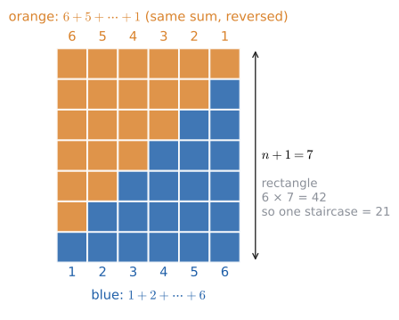
Pairing is fiddly when \(n\) is odd (one number is left unpaired). A cleaner version writes the sum forwards and backwards and adds the two lines:
The picture is even more convincing: a staircase of blocks of heights \(1, 2, \ldots, n\), plus a copy turned upside down, fills an \(n \times (n+1)\) rectangle exactly.
The same "write it twice" argument works for any arithmetic series, because in an arithmetic sequence the first plus the last equals the second plus the second-to-last, and so on (each step forward adds \(d\) to one and subtracts \(d\) from the other):
In words: number of terms times the average of the first and last term. That phrasing is easy to remember and hard to misuse.
|
Triangular numbers
The numbers \(T_n = 1 + 2 + \cdots + n = \frac{n(n+1)}{2}\) (1, 3, 6, 10, 15, …) are the triangular numbers, because that many dots can be arranged in a triangle. Note \(T_n = \binom{n+1}{2}\), the number of ways to choose 2 items from \(n+1\) (Chapter 24). |
14.4.4. The method
Input: first term \(a_1\), common difference \(d\), and either the number of terms \(n\) or the last term \(a_n\).
Steps:
-
If you know the last term but not \(n\), find \(n\) from \(a_n = a_1 + (n-1)d\), i.e. \(n = \frac{a_n - a_1}{d} + 1\).
-
If you know \(n\) but not the last term, compute \(a_n = a_1 + (n-1)d\).
-
Compute \(S_n = \dfrac{n(a_1 + a_n)}{2}\).
-
Sanity-check: \(S_n\) should be \(n\) times something between the smallest and largest term.
Output: the sum \(S_n\).
14.4.5. Worked examples
The whole theatre. 30 rows, \(a_1 = 20\), \(a_{30} = 78\) (found earlier):
Odd numbers. The sum of the first \(n\) odd numbers \(1 + 3 + 5 + \cdots + (2n-1)\): here \(a_1 = 1\), \(a_n = 2n - 1\), so
confirming the "squares are sums of odd numbers" pattern from the start of the chapter.
Sum of multiples. Sum all multiples of 7 between 100 and 500. The first is \(105 = 7\cdot 15\), the last is \(497 = 7 \cdot 71\). Number of terms: \(71 - 15 + 1 = 57\). Sum: \(\frac{57\,(105 + 497)}{2} = \frac{57 \times 602}{2} = 57 \times 301 = 17{,}157\).
14.4.6. Where you’d use this
-
A savings challenge: save $1 in week 1, $2 in week 2, and so on up to $52 in week 52. The total is \(1 + 2 + \cdots + 52 = \tfrac{52 \times 53}{2} = \$1{,}378\). Doing it in reverse (start at $52) gives the same total but front-loads the hard weeks.
-
Sport: in a league where each of \(n\) teams plays every other team once, there are \(0 + 1 + \cdots + (n-1) = \tfrac{n(n-1)}{2}\) fixtures. The Premier League’s 20 teams play home and away, so a season has \(2 \times \tfrac{20 \times 19}{2} = 380\) matches.
-
Physics: a stone dropped from rest falls 4.9 m in the first second, 14.7 m in the next, then 24.5 m, 34.3 m, and so on. That’s an arithmetic sequence with \(d = 9.8\) m (that is, \(g\)). The total after \(n\) seconds is \(\tfrac{n}{2}(4.9 + 4.9(2n-1)) = 4.9n^2\), which is the SUVAT formula \(s = \tfrac12 g t^2\). Galileo noticed the odd-number pattern 1 : 3 : 5 : 7 by rolling balls down ramps.
-
Computing: the running time of every "compare each pair" algorithm is an arithmetic series, as Section 14.9 shows. A 10,000-row table checked pairwise for duplicates needs \(\tfrac{10{,}000 \times 9{,}999}{2} \approx 5 \times 10^7\) comparisons. That is why databases sort or hash instead.
14.4.7. Alternative approach: sums of powers
Gauss’s formula is the first of a family. Others you will occasionally need:
For example \(\sum_{k=1}^{100} k^2 = \frac{100 \cdot 101 \cdot 201}{6} = 338{,}350\). These are best verified by induction (Chapter 22) rather than derived here. For algorithm analysis the takeaway is the pattern: summing \(k^p\) up to \(n\) gives something that grows like \(\frac{n^{p+1}}{p+1}\) — the discrete cousin of \(\int x^p\,dx = \frac{x^{p+1}}{p+1}\) (Chapter 19).
|
Gauss’s formula and the off-by-one
\(\sum_{k=1}^{n} k = \frac{n(n+1)}{2}\) but \(\sum_{k=0}^{n-1} k = \frac{(n-1)n}{2}\). A loop |
14.5. Geometric series: shift and subtract
14.5.1. The problem
You deposit $100 at the end of every year into an account paying 5% annually. How much is there after 10 years? The deposit made at the end of year 10 has earned nothing; the one from year 9 has earned one year’s interest, and so on back to the first deposit, which has earned 9 years. The total is
a geometric series. Gauss’s pairing trick does nothing here — the terms do not pair to a constant. We need a different idea.
14.5.2. Intuition and derivation: shift and subtract
Multiplying a geometric series by its ratio \(r\) shifts every term one place along. Subtracting the shifted copy from the original then cancels almost everything. Let
This is one of the most useful formulas in mathematics. In sigma notation:
The two forms are the same (multiply top and bottom by \(-1\)); use the second when \(r > 1\) to keep things positive. If \(r = 1\) every term is \(a\) and the sum is simply \(na\).
|
Count carefully: the sum has \(n\) terms, from \(ar^0\) to \(ar^{n-1}\), and the exponent in the formula is the number of terms, \(n\), which is one more than the largest exponent. A useful memory aid: "first term times (1 minus ratio to the number-of-terms) over (1 minus ratio)." |
14.5.3. The method
Input: a sum of terms each a constant multiple of the previous one.
Steps:
-
Identify the first term \(a\), the ratio \(r\) (any term divided by the one before), and the number of terms \(n\) (count the exponents: from \(0\) to \(n-1\) is \(n\) terms).
-
If \(r = 1\), return \(na\).
-
Otherwise return \(a\dfrac{1 - r^{n}}{1 - r}\).
-
Sanity-check with \(n = 1\) (should give \(a\)) or by adding the first few terms.
Output: the sum.
def geometric_sum(a, r, n):
    """Sum of the first n terms a + ar + ... + ar^(n-1)."""
    if r == 1:
        return a * n
    return a * (1 - r**n) / (1 - r)

def brute(a, r, n):
    return sum(a * r**k for k in range(n))

for a, r, n in [(3, 2, 10), (1, 0.5, 20), (5, -0.5, 7), (2, 1, 9)]:
    print(a, r, n, geometric_sum(a, r, n), brute(a, r, n))
3 2 10 3069.0 3069 1 0.5 20 1.9999980926513672 1.9999980926513672 5 -0.5 7 3.359375 3.359375 2 1 9 18 18
14.5.4. Worked examples
Savings (an annuity). \(a = 100\), \(r = 1.05\), \(n = 10\):
You deposited $1,000; the other $257.79 is interest on interest.
Powers of two. \(1 + 2 + 4 + \cdots + 2^{n-1}\) has \(a = 1\), \(r = 2\):
So \(1 + 2 + 4 + 8 + 16 + 32 + 64 + 128 = 255 = 2^8 - 1\). Every programmer knows this one in disguise: the largest unsigned 8-bit number, binary 11111111, is \(2^8 - 1\). Notice also that the sum of all the earlier powers of two is one less than the next power. That fact is the engine behind the dynamic-array analysis later in the chapter.
Alternating ratio. \(5 - 2.5 + 1.25 - 0.625 + \cdots\) to 7 terms: \(a = 5\), \(r = -0.5\), \(n = 7\). \((-0.5)^7 = -0.0078125\), so
matching the Python output above.
14.5.5. Where you’d use this
-
Mortgages and loans: a fixed monthly payment \(P\) on a loan of \(L\) at monthly rate \(i\) over \(n\) months must satisfy \(L = P\sum_{k=1}^{n}(1+i)^{-k}\): the loan equals the present value of all the payments. The geometric-series formula turns this into Try it: Mortgage payment and schedule.
\[P = \frac{Li}{1 - (1+i)^{-n}}.\]For a $200,000 mortgage at 4.8% a year (\(i = 0.004\) per month) over 25 years (\(n = 300\)), \(P \approx \$1{,}145.99\) a month. Over the full term you pay about $343,800, so about $143,800 is interest. Every bank’s mortgage calculator is this one line.
-
Pensions: the savings example above is the same formula run forwards. $200 a month for 40 years at 0.5% a month grows to \(200 \cdot \tfrac{1.005^{480} - 1}{0.005} \approx \$398{,}000\), of which only $96,000 was paid in.
-
Computing: a complete binary tree of height \(h\) has \(1 + 2 + \cdots + 2^h = 2^{h+1} - 1\) nodes, so a balanced tree holding a million keys needs only about 20 levels. And the exponential-backoff client above, after 8 failed attempts, has waited \(0.1(1 + 2 + \cdots + 2^7) = 0.1(2^8 - 1) = 25.5\) s in total. That’s the number you put in the timeout configuration.
14.6. Infinite geometric series
14.6.1. The problem: Zeno’s paradox
Around 450 BCE Zeno of Elea argued that motion is impossible. To walk to a wall you must first cover half the distance, then half of what remains, then half of that, and so on — infinitely many tasks. How can infinitely many tasks ever be completed?
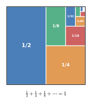
In numbers: the distances are \(\tfrac12, \tfrac14, \tfrac18, \ldots\) of the total, and the question becomes whether
can sensibly have a value. The picture strongly suggests the answer is 1: the pieces tile a unit square ever more completely.
14.6.2. Intuition: watch the partial sums
We cannot literally perform infinitely many additions. What we can do is look at the partial sums and see whether they settle down:
| \(n\) | partial sum \(S_n\) | gap \(1 - S_n\) |
|---|---|---|
1 |
0.5 |
0.5 |
2 |
0.75 |
0.25 |
3 |
0.875 |
0.125 |
5 |
0.96875 |
0.03125 |
10 |
0.9990234375 |
0.0009765625 |
20 |
0.99999904632… |
0.00000095367… |
The gap halves each time. It never becomes exactly zero, but it becomes smaller than any positive tolerance you care to name. That is what we mean when we say the infinite sum equals 1: not that we finish adding, but that the partial sums converge to 1.
14.6.3. Why it works: let n go to infinity in the finite formula
The finite formula already contains the answer. For \(n\) terms,
If \(|r| < 1\), then \(r^{n}\) shrinks towards 0 as \(n\) grows (each multiplication by \(r\) makes it smaller in size). So \(S_n\) approaches \(a \cdot \frac{1 - 0}{1 - r}\):
If \(|r| \ge 1\), \(r^n\) does not shrink, and the partial sums either grow without bound (\(r \ge 1\)), alternate with growing size (\(r < -1\)), or bounce between two values forever (\(r = -1\)). In all these cases the infinite series has no value; we say it diverges.
The phrase "approaches as \(n\) grows" is the idea of a limit, made precise in Chapter 16. For now the intuitive meaning — "gets and stays as close as you like" — is enough.
|
Convergence of a series
An infinite series \(\sum_{k=1}^{\infty} a_k\) converges to \(S\) if its partial sums \(S_n = \sum_{k=1}^{n} a_k\) get arbitrarily close to \(S\) and stay there as \(n \to \infty\) (read "as \(n\) tends to infinity"). We then write \(\sum_{k=1}^{\infty} a_k = S\) and call \(S\) the sum of the series. If the partial sums do not approach any finite number, the series diverges. The symbol \(\infty\) (infinity) here is not a number; \(\sum^{\infty}\) is shorthand for "the limit of the partial sums". |
14.6.4. Worked examples
Zeno. \(a = \tfrac12\), \(r = \tfrac12\): \(\frac{1/2}{1 - 1/2} = 1\). ✓
0.999… = 1. The repeating decimal \(0.\overline{9}\) means the series
Not "infinitely close to 1", not "1 minus a tiny bit": exactly 1. The partial sums \(0.9, 0.99, 0.999, \ldots\) fall short by \(\tfrac{1}{10}, \tfrac{1}{100}, \tfrac{1}{1000}, \ldots\), and the only number they approach is 1.
from fractions import Fraction

# Partial sums of 9/10 + 9/100 + 9/1000 + ...
s = Fraction(0)
for k in range(1, 8):
    s += Fraction(9, 10**k)
    print(k, s, 1 - s)
1 9/10 1/10 2 99/100 1/100 3 999/1000 1/1000 4 9999/10000 1/10000 5 99999/100000 1/100000 6 999999/1000000 1/1000000 7 9999999/10000000 1/10000000
Repeating decimals to fractions. \(0.\overline{27} = 0.272727\ldots = \frac{27}{100} + \frac{27}{100^2} + \cdots\):
This is why every repeating decimal is a rational number (Chapter 1).
The bouncing ball, all the way. Dropped from 10 m, rebounding to 60% each time. The ball falls 10 m, then rises and falls 6 m, rises and falls 3.6 m, and so on:
Achilles and the tortoise. Achilles runs 10 times as fast as a tortoise that starts 100 m ahead. By the time Achilles reaches the tortoise’s start, it has moved 10 m; when he covers that, it has moved 1 m; and so on. Achilles runs \(100 + 10 + 1 + 0.1 + \cdots = \frac{100}{1 - 0.1} = 111.\overline{1}\) m before drawing level — a finite distance, covered in a finite time. Zeno’s infinitely many tasks fit inside a finite total.
14.6.5. Where you’d use this
-
Medicine: you take a 100 mg tablet every morning, and by the next morning your body has cleared half of what was there (a 24-hour half-life). Just after the \(n\)th dose the amount is \(100(1 + 0.5 + 0.5^2 + \cdots + 0.5^{n-1})\): 100, 150, 175, 187.5 mg, and so on. The infinite series gives the long-run peak, \(\frac{100}{1 - 0.5} = 200\) mg, and the trough just before each dose, half that, 100 mg. Pharmacists use exactly this to choose a dose and interval that keep the drug between "effective" and "toxic", and it is why some prescriptions start with a double loading dose: it reaches the steady level on day one.
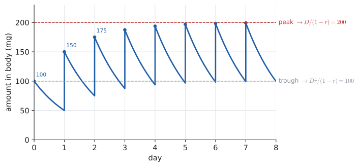 Figure 118. Daily 100 mg doses with half cleared every 24 hours. Each peak is a partial sum of a geometric series, and the peaks approach \(100/(1 - 0.5) = 200\) mg.
-
Economics: if every household spends 80% of any extra income it receives, then $1 of new government spending becomes $0.80 of someone’s income, of which $0.64 is spent again, and so on. The total extra spending is \(1 + 0.8 + 0.64 + \cdots = \frac{1}{1 - 0.8} = \$5\). That’s the Keynesian multiplier.
-
Computing: in reinforcement learning, an agent values a reward that arrives \(k\) steps in the future at \(\gamma^k\) times its face value, with a discount factor \(\gamma\) such as 0.99. A reward of 1 on every step forever is worth \(\sum_{k=0}^{\infty} 0.99^k = \frac{1}{1 - 0.99} = 100\). So \(\frac{1}{1-\gamma}\) acts as the agent’s effective horizon: with \(\gamma = 0.99\) it plans roughly 100 steps ahead.
|
Infinite sums do not behave like finite ones
Applying \(\frac{a}{1-r}\) blindly when \(|r| \ge 1\) gives nonsense. With \(r = 2\): "\(1 + 2 + 4 + 8 + \cdots = \frac{1}{1-2} = -1\)." The partial sums are 1, 3, 7, 15, … and plainly head off to infinity; the formula’s derivation needed \(r^n \to 0\), which is false here. Always check \(|r| < 1\) before using the infinite formula. |
|
Grandi’s series
What is \(1 - 1 + 1 - 1 + 1 - \cdots\)? Grouping as \((1-1) + (1-1) + \cdots\) suggests 0; grouping as \(1 + (-1+1) + (-1+1) + \cdots\) suggests 1; the formula with \(r = -1\) (illegitimately) gives \(\tfrac12\). In 1703 Guido Grandi argued this showed God could create the world from nothing. The modern resolution: the partial sums \(1, 0, 1, 0, \ldots\) never settle, so the series diverges, and regrouping an infinite sum is not a safe operation unless the series converges. (There are more exotic summation methods, used in physics, that do assign it \(\tfrac12\) — but that is a different definition of "sum".) |
|
Geometric series slider
Choose \(a\) and drag a slider for \(r\) from \(-1.5\) to \(1.5\). Plot the partial sums \(S_1, \ldots, S_{40}\) as dots, with a horizontal line at \(\frac{a}{1-r}\) when \(|r| < 1\). Watch the dots zig-zag in when \(r < 0\), creep in slowly when \(r\) is close to 1, and break away to infinity the moment \(|r|\) reaches 1. Try it: Partial sums, slide the ratio |
14.7. Convergence and divergence: a first look
14.7.1. The problem
The geometric series is unusually friendly: we have an exact formula for its partial sums. Most series are not like that. Given \(\sum a_k\), how can we tell whether it converges without a closed form? A full answer belongs to a calculus course, but two facts take you a long way, and one famous example is essential culture.
14.7.2. The divergence test: terms must shrink to zero
If a series converges, its partial sums settle down, so consecutive partial sums get very close together. But \(S_n - S_{n-1} = a_n\). So if \(\sum a_k\) converges, then \(a_k \to 0\). Turned around:
For example, \(\sum_{k=1}^{\infty} \frac{k}{k+1} = \frac12 + \frac23 + \frac34 + \cdots\) diverges, since the terms approach 1: you keep adding almost 1 forever.
The test is one-directional. Terms going to zero is necessary but not sufficient, and the harmonic series is the example everyone should know.
14.7.3. The harmonic series diverges
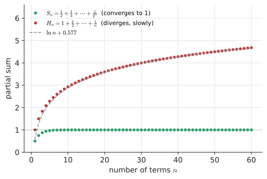
The terms shrink to zero. Surely the sum converges? Compute: after 10 terms it is about 2.93; after 100, about 5.19; after a million, about 14.39. It is growing, but painfully slowly. Is there a ceiling?
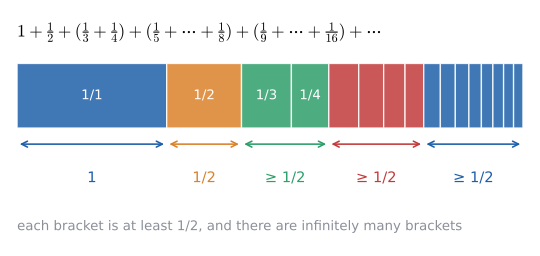
There is not. The proof, due to Nicole Oresme around 1350, is a model of how to bound something you cannot compute: group the terms into blocks that each add up to at least one half.
Block \(m\) contains the \(2^{m-1}\) terms from \(\frac{1}{2^{m-1}+1}\) to \(\frac{1}{2^m}\); each is at least \(\frac{1}{2^m}\), so the block is at least \(2^{m-1}\cdot\frac{1}{2^m} = \frac12\). Adding infinitely many halves exceeds every bound, so the harmonic series diverges. More precisely, the first \(2^m\) terms sum to at least \(1 + \frac{m}{2}\).
|
Grouping consecutive terms of a series of positive terms is safe: it just means looking at a subsequence of the partial sums. The danger shown by Grandi’s series arises with terms of mixed sign. |
14.7.4. How slowly?
The partial sums \(H_n = \sum_{k=1}^{n} \frac1k\) (the harmonic numbers) grow like the natural logarithm: \(H_n \approx \ln n + 0.5772\), where 0.5772… is the Euler–Mascheroni constant \(\gamma\). The reason will be clear once you know that \(\int_1^n \frac{dx}{x} = \ln n\) (Chapter 19). To push the sum past 10 you need more than twelve thousand terms:
import math

H, n, target = 0.0, 0, 10
while H < target:
    n += 1
    H += 1 / n
print(n, H)
print(math.log(n) + 0.5772156649)
12367 10.000043008275778 10.000002578642057
To pass 100 you would need about \(e^{99.42} \approx 1.5 \times 10^{43}\) terms. Divergent, but only just.
14.7.5. Comparison: a first convergence tool
The harmonic proof used an idea worth naming. For series with positive terms, partial sums only go up, so there are just two possibilities: they grow without bound, or they are capped and settle to a limit. Hence the comparison test: if \(0 \le a_k \le b_k\) for every \(k\) and \(\sum b_k\) converges, then \(\sum a_k\) converges too (it is capped by the same ceiling). If \(a_k \ge b_k \ge 0\) and \(\sum b_k\) diverges, so does \(\sum a_k\).
Example. Does \(\sum_{k=1}^{\infty} \frac{1}{2^k + k}\) converge? Each term is smaller than \(\frac{1}{2^k}\), and \(\sum \frac{1}{2^k} = 1\). So yes, and its sum is less than 1.
14.7.6. Where you’d use this
The harmonic numbers \(H_n\) turn up wherever you wait for "the last one of \(n\)".
-
Collecting stickers (the coupon-collector problem): a sticker album has 50 different stickers, and each pack contains one at random. When you already have \(k\) of them, a new pack gives you a new one with probability \((50 - k)/50\), so on average you wait \(50/(50 - k)\) packs for it. The total expected number of packs is
\[\frac{50}{50} + \frac{50}{49} + \cdots + \frac{50}{1} = 50\,H_{50} \approx 50 \times 4.499 \approx 225.\]Nearly a quarter of that is spent on the last four stickers (\(50(1 + \tfrac12 + \tfrac13 + \tfrac14) \approx 104\) packs). That is why the last few are so annoying, and why sticker swaps exist.
-
Physics and engineering: stack identical books at the edge of a table, each sticking out as far as it can without toppling. With \(n\) books the top one can overhang by \(\tfrac12 H_n\) book lengths. Four books give \(\tfrac12(1 + \tfrac12 + \tfrac13 + \tfrac14) \approx 1.04\), so the top book sits entirely beyond the table edge. Because \(H_n\) diverges, a tall enough stack could reach any distance at all, but slowly: an overhang of 3 lengths needs 227 books.
-
Computing: the coupon-collector bound tells you how many random requests it takes before a load balancer has hit all \(n\) servers, or how many random tests are needed before every one of \(n\) code paths has been exercised: about \(n \ln n\). The same \(\ln n\) from harmonic sums gives the average cost of quicksort, about \(2n\ln n\) comparisons.
|
Basel problem
Squaring the denominators changes everything: \(\sum_{k=1}^{\infty} \frac{1}{k^2}\) converges. Finding its exact value defeated the best mathematicians for decades until Leonhard Euler announced in 1734 that
\[1 + \frac14 + \frac19 + \frac{1}{16} + \cdots = \frac{\pi^2}{6}.\]
Why should \(\pi\), a circle number, appear in a sum of reciprocal squares? Euler’s argument treated \(\frac{\sin x}{x}\) as an "infinite polynomial" with roots at \(\pm\pi, \pm 2\pi, \ldots\). More generally \(\sum \frac{1}{k^p}\) converges exactly when \(p > 1\); the harmonic series sits right on the knife-edge \(p = 1\). |
|
When to trust a computed sum
You cannot decide convergence by computing. Summing the harmonic series in double-precision floating point eventually stalls: once \(H_n\) reaches about 34 (after roughly \(2^{48}\) terms), adding \(1/n\) changes nothing in the last bit, and a naive program would report a "limit". Conversely, a convergent series like \(\sum (-1)^{k+1}/k\) (which equals \(\ln 2\)) converges so slowly that a million terms gives only about six correct digits. Use mathematics to decide whether a sum converges, and computation to estimate what it converges to (Chapter 32). |
14.8. Recurrence relations
14.8.1. The problem
Many sequences arise naturally as recurrences, and for many of them no one hands you an explicit formula. The Tower of Hanoi puzzle moves \(n\) disks between three pegs, never placing a larger disk on a smaller. To move \(n\) disks you must move the top \(n-1\) out of the way, move the largest disk, and then move the \(n-1\) back on top. So the minimum number of moves \(h_n\) satisfies
How many moves for 64 disks? You do not want to iterate 64 times by hand, and you certainly want to know the growth rate.
|
Recurrence relation and order
A recurrence relation defines each term of a sequence from earlier terms. Its order is how far back it reaches: \(a_n = 3a_{n-1}\) is first order, \(F_n = F_{n-1} + F_{n-2}\) is second order. An order-\(k\) recurrence needs \(k\) initial conditions. Solving a recurrence means finding an explicit formula for \(a_n\). |
14.8.2. Method 1: unroll and spot the pattern
Substitute the recurrence into itself repeatedly:
Check: \(h_1 = 1\), \(h_2 = 3\), \(h_3 = 7\). ✓ For 64 disks, \(2^{64} - 1 \approx 1.8 \times 10^{19}\) moves; at one per second that is about 585 billion years. Notice how the geometric series appeared in the middle of the unrolling — this happens constantly.
14.8.3. Method 2: guess and verify
If you suspect a form, check it satisfies both the recurrence and the initial condition. Guess \(h_n = 2^n - 1\): then \(2h_{n-1} + 1 = 2(2^{n-1} - 1) + 1 = 2^n - 2 + 1 = 2^n - 1 = h_n\) ✓, and \(h_1 = 2 - 1 = 1\) ✓. This "verify" step is essentially a proof by induction (Chapter 22).
Input: a recurrence \(a_n = c\,a_{n-1} + g(n)\) and an initial value.
Steps:
-
Substitute the recurrence for \(a_{n-1}\), then for \(a_{n-2}\), and so on, writing out three or four levels in full.
-
Spot the pattern after \(j\) levels: typically \(a_n = c^{j}a_{n-j} + (\text{a sum of } j \text{ terms})\).
-
Choose \(j\) so that \(a_{n-j}\) is the initial value.
-
Evaluate the remaining sum in closed form (it is often arithmetic or geometric).
-
Verify the formula on the first two or three terms.
Output: an explicit formula for \(a_n\).
14.8.4. Fibonacci numbers
The most famous recurrence is second order:
giving \(0, 1, 1, 2, 3, 5, 8, 13, 21, 34, 55, \ldots\). Leonardo of Pisa (Fibonacci) introduced it in 1202 as an idealised rabbit-breeding puzzle, but it turns up in plant spirals, in the analysis of Euclid’s algorithm (Chapter 23), and in counting problems: \(F_{n+1}\) is the number of ways to tile a \(1 \times n\) strip with squares and dominoes.
Ratios of consecutive terms. Compute \(F_{n+1}/F_n\): \(1, 2, 1.5, 1.667, 1.6, 1.625, 1.615, 1.619, 1.6176, 1.6182, \ldots\) The ratios settle to a limit. If the ratio approaches some \(\varphi\), then for large \(n\), \(F_n \approx \varphi F_{n-1}\) and \(F_{n-1} \approx \varphi F_{n-2}\); substituting into the recurrence and dividing by \(F_{n-2}\):
(The quadratic formula is derived in Chapter 8.) This is the golden ratio. The same quadratic (called the characteristic equation) leads to the exact closed form, Binet’s formula:
Since \(|\psi| < 1\), the \(\psi^n\) term shrinks to nothing, and \(F_n\) is simply \(\varphi^n/\sqrt5\) rounded to the nearest integer. For instance, \(\varphi^{20}/\sqrt5 \approx 6765.00003\), and \(F_{20} = 6765\). The upshot: Fibonacci numbers grow exponentially, by a factor of about 1.618 per step. (The general technique for linear recurrences, using the characteristic equation, is best seen through eigenvalues: Chapter 28.)
|
The golden ratio is overrated (a bit)
The golden ratio really does appear in sunflower seed heads and pine cones, where successive seeds are placed about \(360^\circ/\varphi^2 \approx 137.5^\circ\) apart — the angle that packs them most evenly. But many popular claims (the Parthenon, the Mona Lisa, "the most pleasing rectangle") do not survive measurement. In mathematics its fame is deserved for a different reason: \(\varphi\) is, in a precise sense, the irrational number hardest to approximate by fractions, because its continued fraction is \(1 + \cfrac{1}{1 + \cfrac{1}{1 + \cdots}}\). |
14.8.5. Worked example: a recurrence from a story
A population of fish is 2,000. Each year it grows by 10% and then 150 fish are harvested. Find a formula for the population \(p_n\) after \(n\) years.
Set up. \(p_0 = 2000\), \(p_n = 1.1\,p_{n-1} - 150\).
Unroll.
Check. \(p_0 = 500 + 1500 = 2000\) ✓. \(p_1 = 1.1(2000) - 150 = 2050\); formula: \(550 + 1500 = 2050\) ✓.
Interpret. 1500 is the equilibrium (if \(p = 1500\), then \(1.1p - 150 = 1500\) again). Starting above it, the population grows exponentially away from it; starting below it, the harvest would drive the population to zero. A single closed form reveals behaviour the recurrence hides.
14.8.6. Where you’d use this
-
Credit cards and loans: you owe $1,000 at 2% interest a month and pay $50 a month. The balance obeys \(b_n = 1.02\,b_{n-1} - 50\) with \(b_0 = 1000\). Unrolling exactly as for the fish gives \(b_n = 2500 - 1500(1.02)^n\), which reaches zero when \(1.02^n = \tfrac53\), at \(n = \ln(5/3)/\ln 1.02 \approx 25.8\), so you’re clear in 26 months. The equilibrium is the warning sign: at $20 a month the equilibrium is \(20/0.02 = \$1{,}000\), your current balance, so you would pay forever and never reduce the debt.
-
Biology and ecology: the fish model is a real tool for setting fishing quotas, and the same first-order recurrences describe drug clearance, cell cultures and invasive species.
-
Computing: the next section is entirely about recurrences in software: loops, growable arrays, divide-and-conquer and memoisation.
14.9. Sums and recurrences in algorithm analysis
This section gathers the computing payoffs. Each one is a direct application of something above.
14.9.1. Loops are sums
The running time of a loop is the sum, over iterations, of the work done in each iteration. Consider checking every unordered pair of \(n\) items (for duplicate detection, collision tests, or a naive closest-pair search):
def count_pairs(n):
    ops = 0
    for i in range(n):
        for j in range(i + 1, n):   # every unordered pair (i, j) with i < j
            ops += 1
    return ops

for n in [10, 100, 1000]:
    print(n, count_pairs(n), n * (n - 1) // 2)
10 45 45 100 4950 4950 1000 499500 499500
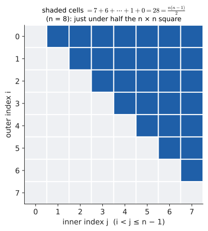
Translate the loop into a sum. For a fixed \(i\), the inner loop runs for \(j = i+1, \ldots, n-1\), which is \(n - 1 - i\) iterations. So
That is \(\frac12 n^2 - \frac12 n\). For large \(n\) the \(n^2\) term dominates, so we say the loop is \(O(n^2)\) ("order \(n\) squared"): doubling \(n\) roughly quadruples the work. The triangle-shaped loop does half the work of a full \(n \times n\) double loop, but halving does not change the growth rate. The precise meaning of \(O(\cdot)\) as a statement about limits is in Chapter 16.
14.9.2. Dynamic arrays: why append is O(1) on average
Python lists, Java ArrayList, C++ std::vector, and Go slices all grow by doubling: when the array is full, allocate one twice as big and copy everything across. Copying is expensive, so how can appending be "constant time"? Try it: Dynamic array amortised cost.
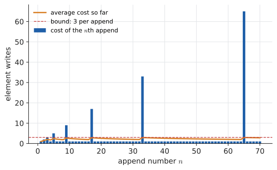
Count element writes for \(n\) appends, starting from capacity 1. Every append writes one new element: \(n\) writes. Resizes happen when the size reaches 1, 2, 4, 8, …, copying that many elements. If the largest resize copies \(2^m\) elements, where \(2^m < n\), the total copying is a geometric series:
So the total work is less than \(n + 2n = 3n\): fewer than 3 writes per append on average, however large \(n\) grows. This "average over a sequence of operations" is called amortised cost. The key is the powers-of-two fact: the sum of all previous resizes is smaller than the latest one.
class DynamicArray:
    def __init__(self):
        self.capacity, self.size = 1, 0
        self.data = [None]
        self.writes = 0              # count every element written

    def append(self, x):
        if self.size == self.capacity:
            self.capacity *= 2
            new = [None] * self.capacity
            for i in range(self.size):   # copy the old contents
                new[i] = self.data[i]
                self.writes += 1
            self.data = new
        self.data[self.size] = x
        self.size += 1
        self.writes += 1

for n in [10, 1000, 1_000_000]:
    arr = DynamicArray()
    for k in range(n):
        arr.append(k)
    print(n, arr.writes, round(arr.writes / n, 3))
10 25 2.5 1000 2023 2.023 1000000 2048575 2.049
|
Grow by a constant amount and you lose
Suppose instead the array grows by a fixed 100 slots each time. Resizes copy 100, 200, 300, … elements — an arithmetic series. After \(n\) appends there have been about \(n/100\) resizes, costing about \(100 \cdot \frac{(n/100)^2}{2} = \frac{n^2}{200}\) copies: \(O(n^2)\) total, \(O(n)\) per append on average. Arithmetic growth leads to quadratic cost; geometric growth leads to linear cost. Any factor greater than 1 works (CPython uses about 1.125, many C++ libraries 1.5 or 2), trading wasted memory for fewer copies. |
14.9.3. Divide-and-conquer recurrences
Merge sort splits an array in half, sorts each half recursively, and merges the halves in linear time. Its cost satisfies, informally (for \(n\) a power of 2, measuring cost in units where merging \(n\) items costs \(n\)), Try it: Merge-sort recursion tree.
Unroll it exactly as we did for Hanoi:
The recursion bottoms out when \(n/2^k = 1\), i.e. \(k = \log_2 n\) (Chapter 12). Then
Picture a recursion tree: \(\log_2 n\) levels, each doing \(n\) total work. That is where the ubiquitous \(O(n \log n)\) comes from. Compare the recurrence \(T(n) = T(n/2) + 1\) (binary search: one half discarded, constant work), which unrolls to \(\log_2 n\), and \(T(n) = 2T(n/2) + 1\) (visiting every node of a balanced tree), which unrolls to a geometric series \(1 + 2 + 4 + \cdots + n/2 \approx n\). The general pattern is captured by the "master theorem" in algorithms textbooks; behind it are nothing but geometric series.
import math

def T(n):
    """T(n) = 2 T(n/2) + n, T(1) = 0, for n a power of 2."""
    if n == 1:
        return 0
    return 2 * T(n // 2) + n

for k in [1, 4, 10, 20]:
    n = 2**k
print(n, T(n), n * int(math.log2(n)))2 2 2 16 64 64 1024 10240 10240 1048576 20971520 20971520
14.9.4. Fibonacci: recursion versus memoisation
Translate the Fibonacci recurrence literally into code and you get something correct but catastrophically slow:
from functools import lru_cache

calls = 0
def fib_naive(n):
    global calls
    calls += 1
    if n < 2:
        return n
    return fib_naive(n - 1) + fib_naive(n - 2)

@lru_cache(maxsize=None)
def fib_memo(n):
    if n < 2:
        return n
    return fib_memo(n - 1) + fib_memo(n - 2)

def fib_iter(n):
    a, b = 0, 1
    for _ in range(n):
        a, b = b, a + b
    return a

print(fib_naive(25), calls)
print(fib_memo(25), fib_memo.cache_info().misses)
print(fib_iter(100))
75025 242785 75025 26 354224848179261915075
Why 242,785 calls? Let \(C_n\) be the number of calls made by fib_naive(n). Then \(C_0 = C_1 = 1\) and \(C_n = 1 + C_{n-1} + C_{n-2}\) — the call count obeys a Fibonacci-like recurrence itself. Its solution is \(C_n = 2F_{n+1} - 1\) (check: \(2F_{26} - 1 = 2(121{,}393) - 1 = 242{,}785\)). So the cost grows like \(\varphi^n \approx 1.618^n\): exponential. The call tree shows why: the same subproblems are recomputed again and again.
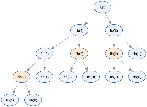
Memoisation caches each result the first time it is computed, so each \(F_k\) is computed once: 26 distinct computations for \(n = 25\), linear in \(n\). The iterative version goes further and keeps only the last two values — the recurrence evaluated "bottom up". That move from top-down recursion with a cache to bottom-up iteration over a table is the essence of dynamic programming. Try it: Call tree of fib(5).
|
Visualise the waste
Animate the call tree of |
|
Gauss’s staircase, live
Drag a slider for \(n\) and watch two staircases of 1 to \(n\) blocks slide together into an \(n \times (n+1)\) rectangle. A second mode shows the nested-loop grid filling cell by cell as a program runs, with a running counter matching \(\frac{n(n-1)}{2}\). |
14.10. Interactive tools
Browser tools on the companion website that go with this chapter. Each example link in the chapter opens one of them with that example already set up.
14.11. Exercises
Recognition
-
Classify each as arithmetic, geometric, or neither, and give \(a_n\) if possible: (a) \(4, 1, -2, -5, \ldots\) (b) \(48, 12, 3, \tfrac34, \ldots\) (c) \(1, 4, 9, 16, \ldots\) (d) \(2, -6, 18, -54, \ldots\).
-
Write out every term and evaluate: (a) \(\sum_{k=1}^{4} k^3\) (b) \(\sum_{j=0}^{3} (-2)^j\) (c) \(\prod_{i=1}^{4} \frac{i}{i+1}\) (d) \(\sum_{i=5}^{3} i\).
-
Write in sigma notation: (a) \(3 + 6 + 9 + \cdots + 300\) (b) \(1 - \tfrac13 + \tfrac15 - \tfrac17 + \cdots - \tfrac{1}{99}\).
Application
-
Find the sum of all three-digit odd numbers.
-
A job offer starts at $60,000 with a 3% raise every year. What are total earnings over the first 20 years? (Give the closed form and a numerical value.)
-
Telescoping. Use \(\frac{1}{k(k+1)} = \frac1k - \frac{1}{k+1}\) to evaluate \(\sum_{k=1}^{n} \frac{1}{k(k+1)}\), and hence the infinite sum.
-
Convert \(0.4\overline{6} = 0.4666\ldots\) and \(1.\overline{142857}\) into fractions.
-
Does each converge? If so, find the sum. (a) \(\sum_{k=0}^{\infty} 5\left(-\tfrac23\right)^k\) (b) \(\sum_{k=1}^{\infty} \left(\tfrac{5}{4}\right)^k\) (c) \(\sum_{k=1}^{\infty} \frac{2k}{3k+1}\) (d) \(\sum_{k=1}^{\infty} \frac{1}{3^k + 1}\).
Problem solving
-
Solve the recurrence \(a_0 = 5\), \(a_n = 3a_{n-1} - 4\) by unrolling. Verify for \(n = 1, 2\).
-
How many times does the innermost statement run, as an exact function of \(n\)?
for i in range(n): for j in range(i): for k in range(j): work() -
Show that \(\sum_{k=1}^{\infty} \frac{1}{2k}\) diverges using the harmonic series, and explain why \(\sum_{k=1}^{\infty} \frac{1}{k\cdot 2^k}\) converges.
-
A recursive algorithm satisfies \(T(1) = 1\), \(T(n) = 3T(n/3) + n\) for \(n\) a power of 3. Unroll to find \(T(n)\) exactly.
Answers
-
(a) Arithmetic, \(d = -3\): \(a_n = 4 - 3(n-1) = 7 - 3n\). (b) Geometric, \(r = \tfrac14\): \(a_n = 48\left(\tfrac14\right)^{n-1}\). (c) Neither (differences 3, 5, 7; ratios 4, 2.25, 1.78): \(a_n = n^2\). (d) Geometric, \(r = -3\): \(a_n = 2(-3)^{n-1}\).
-
(a) \(1 + 8 + 27 + 64 = 100\) (and \(100 = (\tfrac{4\cdot5}{2})^2\), as the sum-of-cubes formula predicts). (b) \(1 - 2 + 4 - 8 = -5\). (c) \(\tfrac12\cdot\tfrac23\cdot\tfrac34\cdot\tfrac45 = \tfrac15\) (everything cancels except the first numerator and last denominator). (d) Upper bound below lower bound: empty sum, 0.
-
(a) \(\sum_{k=1}^{100} 3k\). (b) The denominators are odd: \(2k-1\) for \(k = 1, \ldots, 50\) (since \(2\cdot50 - 1 = 99\)); signs alternate starting positive: \(\sum_{k=1}^{50} \frac{(-1)^{k+1}}{2k-1}\).
-
Odd three-digit numbers: \(101, 103, \ldots, 999\). \(d = 2\), \(n = \frac{999 - 101}{2} + 1 = 450\). \(S = \frac{450(101 + 999)}{2} = 450 \times 550 = 247{,}500\).
-
Geometric with \(a = 60000\), \(r = 1.03\), \(n = 20\): \(S = 60000\cdot\frac{1.03^{20} - 1}{0.03}\). \(1.03^{20} \approx 1.806111\), so \(S \approx 60000 \times 26.8704 \approx \$1{,}612{,}222\).
-
\(\sum_{k=1}^{n}\left(\frac1k - \frac1{k+1}\right) = \left(1 - \tfrac12\right) + \left(\tfrac12 - \tfrac13\right) + \cdots + \left(\tfrac1n - \tfrac1{n+1}\right)\). Each negative term cancels the next positive term ("telescopes"), leaving \(1 - \frac{1}{n+1} = \frac{n}{n+1}\). As \(n \to \infty\) this approaches 1, so the infinite sum is 1.
-
\(0.4\overline{6} = \tfrac{4}{10} + \left(\tfrac{6}{100} + \tfrac{6}{1000} + \cdots\right) = \tfrac{4}{10} + \frac{6/100}{1 - 1/10} = \tfrac{4}{10} + \tfrac{6}{90} = \tfrac{36}{90} + \tfrac{6}{90} = \tfrac{42}{90} = \tfrac{7}{15}\). \(1.\overline{142857} = 1 + \frac{142857/10^6}{1 - 10^{-6}} = 1 + \frac{142857}{999999} = 1 + \frac17 = \frac87\).
-
(a) \(|r| = \tfrac23 < 1\): converges to \(\frac{5}{1 + 2/3} = \frac{5}{5/3} = 3\). (b) \(r = \tfrac54 > 1\): diverges. (c) Terms approach \(\tfrac23 \ne 0\): diverges by the divergence test. (d) \(0 < \frac{1}{3^k+1} < \frac{1}{3^k}\) and \(\sum_{k\ge1} 3^{-k} = \frac{1/3}{1 - 1/3} = \tfrac12\): converges by comparison, to something less than \(\tfrac12\).
-
\(a_n = 3a_{n-1} - 4 = 9a_{n-2} - 4(3 + 1) = \cdots = 3^n a_0 - 4(3^{n-1} + \cdots + 3 + 1) = 5\cdot3^n - 4\cdot\frac{3^n - 1}{2} = 5\cdot 3^n - 2\cdot 3^n + 2 = 3^{n+1} + 2\). Check: \(a_1 = 3\cdot5 - 4 = 11 = 9 + 2\) ✓; \(a_2 = 3\cdot11 - 4 = 29 = 27 + 2\) ✓. (Equilibrium is \(a = 3a - 4 \Rightarrow a = 2\), visible in the formula.)
-
For fixed \(i\) and \(j\), the inner loop runs \(j\) times. Summing over \(j < i\): \(\sum_{j=0}^{i-1} j = \frac{i(i-1)}{2}\). Then summing over \(i\): \(\sum_{i=0}^{n-1}\frac{i(i-1)}{2}\). This counts triples \(k < j < i\) chosen from \(\{0, \ldots, n-1\}\), which is \(\binom{n}{3} = \frac{n(n-1)(n-2)}{6}\). (Check \(n = 4\): \(i = 2\) contributes 1, \(i = 3\) contributes 3, total 4 = \(\binom43\) ✓.) It is \(O(n^3)\).
-
\(\sum \frac{1}{2k} = \frac12 \sum \frac1k\); half of something that grows without bound also grows without bound, so it diverges. For the second, \(0 < \frac{1}{k 2^k} \le \frac{1}{2^k}\) and \(\sum \frac{1}{2^k}\) converges (to 1), so it converges by comparison. (Its sum is in fact \(\ln 2\).)
-
\(T(n) = 3T(n/3) + n = 9T(n/9) + 2n = \cdots = 3^k T(n/3^k) + kn\). With \(k = \log_3 n\): \(T(n) = n\cdot T(1) + n\log_3 n = n + n\log_3 n\). Check \(n = 3\): \(3T(1) + 3 = 6 = 3 + 3\cdot1\) ✓.
14.12. Mastery check
-
Find the 40th term and the sum of the first 40 terms of \(-3, 2, 7, 12, \ldots\).
-
Evaluate \(\sum_{k=1}^{20}(4k - 1)\) using the sigma rules (show the split).
-
Derive the formula for \(1 + r + r^2 + \cdots + r^{n-1}\) by shift-and-subtract, then use it to compute \(\sum_{k=0}^{9} 3^k\).
-
Express \(0.\overline{81}\) as a fraction in lowest terms.
-
Explain in two or three sentences why \(\sum \frac{1}{k}\) diverges even though \(\frac1k \to 0\).
-
A loop
for i in range(1, n+1): for j in range(i, n+1): work()— exactly how many calls towork()? -
Solve \(a_1 = 2\), \(a_n = a_{n-1} + 3n\). (Hint: unroll to a sum and use the sigma rules.)
Decision rule: All correct without hesitation → move on to Chapter 15 (or Chapter 16 if complex numbers are already solid). Stuck on 1–2 → reread Section 14.4 and Section 14.5. Stuck on 5 → reread Section 14.7. Stuck on 6–7 → work through Section 14.9 and Section 14.8, then the section exercises.
Mastery check answers
-
\(a_1 = -3\), \(d = 5\): \(a_{40} = -3 + 39\cdot5 = 192\). \(S_{40} = \frac{40(-3 + 192)}{2} = 20 \times 189 = 3780\).
-
\(\sum_{k=1}^{20}(4k - 1) = 4\sum_{k=1}^{20}k - \sum_{k=1}^{20}1 = 4\cdot\frac{20\cdot21}{2} - 20 = 840 - 20 = 820\).
-
\(S = 1 + r + \cdots + r^{n-1}\), \(rS = r + \cdots + r^{n}\); subtract: \(S - rS = 1 - r^n\), so \(S = \frac{1 - r^n}{1 - r}\) for \(r \ne 1\). With \(r = 3\), \(n = 10\): \(\frac{3^{10} - 1}{3 - 1} = \frac{59049 - 1}{2} = 29{,}524\).
-
\(\frac{81/100}{1 - 1/100} = \frac{81}{99} = \frac{9}{11}\).
-
Group the terms into blocks \(\left(\tfrac13 + \tfrac14\right), \left(\tfrac15 + \cdots + \tfrac18\right), \ldots\); block \(m\) has \(2^{m-1}\) terms each at least \(1/2^m\), so each block is at least \(\tfrac12\). Infinitely many blocks each worth at least \(\tfrac12\) add up to more than any bound. The terms shrink, but not fast enough: you keep finding another half.
-
For each \(i\), the inner loop runs \(n - i + 1\) times. \(\sum_{i=1}^{n}(n - i + 1) = n + (n-1) + \cdots + 1 = \frac{n(n+1)}{2}\).
-
\(a_n = a_1 + \sum_{k=2}^{n} 3k = 2 + 3\left(\frac{n(n+1)}{2} - 1\right) = \frac{3n(n+1)}{2} - 1\). Check: \(a_1 = 3 - 1 = 2\) ✓, \(a_2 = 2 + 6 = 8 = 9 - 1\) ✓, \(a_3 = 8 + 9 = 17 = 18 - 1\) ✓.