Volume 2: Continuous Mathematics · Part V: Calculus
Chapter 19. The Integral
Chapter map. The derivative answered "how fast is this changing right now?" This chapter answers the reverse question: "if I know how fast something changes at every instant, how much has it changed in total?" We start with a car whose speed keeps changing and ask how far it travelled. That question turns into the area under a curve. We approximate the area with rectangles (Riemann sums), push the approximation to a limit (the definite integral), and then meet the result that ties all of calculus together: the Fundamental Theorem of Calculus, which says integration is differentiation run backwards. After that come the techniques (antiderivatives, substitution, integration by parts), the applications (areas, averages, volumes, work, probability), integrals over infinite ranges, numerical integration for when the algebra gives up, and a first look at differential equations, which is how physics engines and population models actually run.
Why this chapter matters: whenever you know a rate and want a total, you are integrating. Your electricity bill is the integral of power over the month; a fitness tracker’s distance is the integral of speed; a drug’s total exposure is the area under its concentration curve; a cloud bill is the integral of usage over time; a game advances its world by integrating velocity every frame. Probability for continuous quantities is defined as area, which is why the integral underpins statistics and machine learning too.
19.1. The problem: how far did the car go?
19.1.1. Constant speed is easy
If a car drives at a steady 60 mph for 2 hours it covers \(60 \times 2 = 120\) miles. Draw that on a graph with time across and speed up, and the journey is a horizontal line at height 60 running from \(t = 0\) to \(t = 2\). The distance, 120, is the area of the rectangle under that line: height (speed) times width (time).
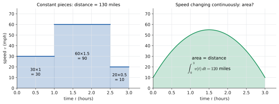
Now let the speed change in jumps. Say 30 mph for the first hour, 60 mph for the next 1.5 hours, then 20 mph for the last half hour. Each piece is a rectangle, and the total distance is the sum of their areas:
19.1.2. Changing speed is the real problem
Real cars do not change speed in jumps. Suppose the speed in mph after \(t\) hours is
It starts at 10 mph, peaks at 55 mph at \(t = 1.5\), and falls back to 10 mph. How far did the car go?
There is no single speed to multiply by 3 hours. But the rectangle picture suggests what to do. On a short enough time interval the speed hardly changes, so "speed times time" is nearly right for that sliver. Chop the journey into many slivers, treat the speed as constant on each, add up the little distances, and make the slivers thinner and thinner. That is the whole idea of the integral, and it is the same limiting move you met with derivatives, applied to a sum instead of a ratio.
Notice what has happened. We started with a physical question (distance from speed) and ended with a geometric one (the area under a curve). These are the same problem, and the integral is the tool that answers both. By the end of the section on the Fundamental Theorem we will find that this car covered exactly 120 miles.
Notice too how this reverses the previous chapter. There, position \(s(t)\) was given and we differentiated to get speed \(v(t) = s'(t)\). Here the speed is given and we want the change in position. Integration will turn out to be the inverse of differentiation, which is why it is sometimes called antidifferentiation.
|
Accumulation
An accumulated quantity is a total built up from a rate over time (or over any other variable). Distance accumulates from speed, water in a tank accumulates from flow rate, money accumulates from income per month. If the rate is constant, total = rate × duration. If the rate varies, total = area under the rate graph. The integral is the tool for computing that area. |
19.2. Riemann sums: rectangles under a curve
19.2.1. The idea
Take the simplest curved example: the area under \(y = x^2\) between \(x = 0\) and \(x = 2\). No school formula gives this region’s area: it is not a triangle, rectangle or circle segment. So we approximate it.
Cut the interval \({[0, 2]}\) into \(n\) equal pieces. Above each piece, build a rectangle whose height is the curve’s height somewhere in that piece. Add the rectangle areas. The choice of "somewhere" gives three standard versions:
-
Left sum: use the height at the left end of each piece.
-
Right sum: use the height at the right end.
-
Midpoint sum: use the height at the middle.
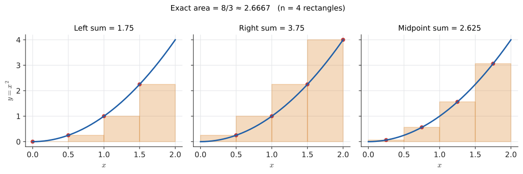
Because \(x^2\) is increasing on this interval, the left sum leaves gaps under the curve (an underestimate) and the right sum overshoots (an overestimate). The midpoint sum overshoots on half of each piece and undershoots on the other half, so the errors largely cancel.
19.2.2. Vocabulary and notation
|
Partition, subinterval, width
A partition of \({[a, b]}\) splits it into smaller subintervals using points \(a = x_0 < x_1 < \dots < x_n = b\). With equal widths, each subinterval has width
\[\Delta x = \frac{b - a}{n},\]
and the partition points are \(x_i = a + i\,\Delta x\) for \(i = 0, 1, \dots, n\). The symbol \(\Delta\) ("delta") means "a change in", so \(\Delta x\) is read "delta x": a small step in \(x\). |
|
Sample point
A sample point \(x_i^*\) (read "x i star") is the point inside the \(i\)-th subinterval where you measure the height \(f(x_i^*)\). Left, right and midpoint sums are three particular choices of sample point. |
|
Sigma notation
The capital Greek letter \(\Sigma\) (sigma, for "sum") abbreviates a long addition:
\[\sum_{i=1}^{n} f(x_i^*)\,\Delta x \;=\; f(x_1^*)\,\Delta x + f(x_2^*)\,\Delta x + \dots + f(x_n^*)\,\Delta x.\]
Piece by piece: \(i\) is the index (a loop counter); \(i = 1\) underneath is where it starts; \(n\) on top is where it stops (inclusive); the expression to the right is the term evaluated for each \(i\) and then added. In code it is |
|
Riemann sum
A Riemann sum for \(f\) on \({[a, b]}\) is any sum of the form \(\sum_{i=1}^{n} f(x_i^*)\,\Delta x\): heights times widths, added. Each term is the (signed) area of one thin rectangle. Named after Bernhard Riemann (1826–1866), who made the definition precise. |
19.2.3. Worked example: three sums by hand
Approximate the area under \(f(x) = x^2\) on \({[0, 2]}\) using \(n = 4\). Try it: Draw the three sums; Watch the rectangles.
Step 1: the width. \(\Delta x = (2 - 0)/4 = 0.5\).
Step 2: the partition points. \(x_0 = 0,\ x_1 = 0.5,\ x_2 = 1,\ x_3 = 1.5,\ x_4 = 2.\)
Step 3: left sum. Heights at \(0, 0.5, 1, 1.5\):
Step 4: right sum. Heights at \(0.5, 1, 1.5, 2\):
Step 5: midpoint sum. Midpoints are \(0.25, 0.75, 1.25, 1.75\):
The true area, as we will soon prove, is \(8/3 \approx 2.6667\). The midpoint sum is already within 0.042 of it with only four rectangles; the left and right sums are off by about 0.92 and 1.08.
Input: a function \(f\), an interval \({[a, b]}\), a number of subintervals \(n\), and a rule (left, right or midpoint).
Steps:
-
Compute the width \(\Delta x = (b - a)/n\).
-
For each \(i = 0, 1, \dots, n-1\), choose the sample point: \(a + i\Delta x\) (left), \(a + (i+1)\Delta x\) (right), or \(a + (i + \tfrac12)\Delta x\) (midpoint).
-
Evaluate \(f\) at each sample point.
-
Add the heights and multiply the total by \(\Delta x\).
Output: an approximation to the area under \(f\) on \({[a, b]}\). It improves as \(n\) grows.
def riemann_sum(f, a, b, n, rule="mid"):
    """Approximate the integral of f on [a, b] with n rectangles."""
    dx = (b - a) / n
    offset = {"left": 0.0, "right": 1.0, "mid": 0.5}[rule]
    total = 0.0
    for i in range(n):
        x_sample = a + (i + offset) * dx   # where we measure the height
        total += f(x_sample) * dx          # height times width
    return total

f = lambda x: x**2
for n in [4, 16, 64, 256, 1024]:
    print(f"n={n:5d}  left={riemann_sum(f,0,2,n,'left'):.6f}  "
          f"right={riemann_sum(f,0,2,n,'right'):.6f}  "
          f"mid={riemann_sum(f,0,2,n,'mid'):.6f}")
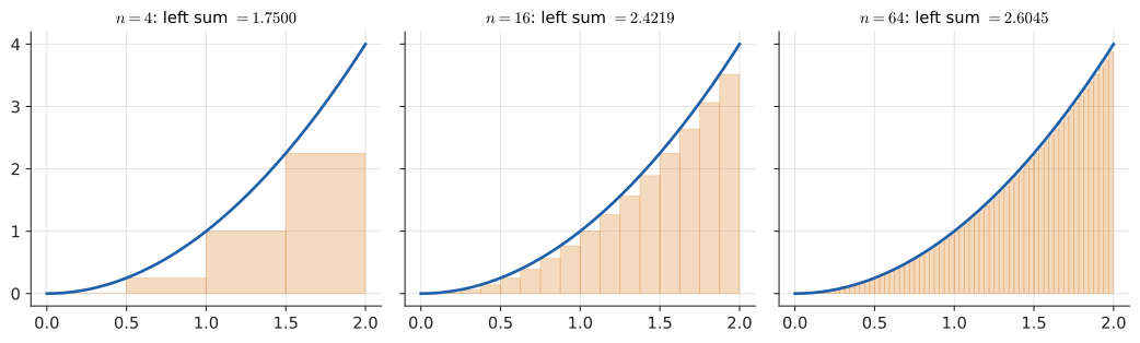
n= 4 left=1.750000 right=3.750000 mid=2.625000 n= 16 left=2.421875 right=2.921875 mid=2.664062 n= 64 left=2.604492 right=2.729492 mid=2.666504 n= 256 left=2.651062 right=2.682312 mid=2.666656 n= 1024 left=2.662762 right=2.670574 mid=2.666666
All three columns close in on \(2.6666\ldots\). Look at the rates: each time \(n\) is multiplied by 4, the left and right errors shrink by roughly a factor of 4, while the midpoint error shrinks by roughly 16. The midpoint rule is not just a little better; it improves faster. We will see why in Section 19.12.
19.2.4. Why it works: the exact limit by algebra
For this one function we can compute the sum exactly for every \(n\) and watch the limit happen. Use right endpoints: \(\Delta x = 2/n\) and \(x_i = 2i/n\), so \(f(x_i) = 4i^2/n^2\).
Check with \(n = 4\): \(\tfrac43 \times 1.25 \times 2.25 = 3.75\), matching the hand calculation. As \(n \to \infty\), both \(1/n\) terms vanish and
That is a genuine derivation of the area under a parabola. It also shows why we need something better: this needed a special formula for \(\sum i^2\), and a function like \(\sin x\) or \(e^{-x^2}\) has no such convenient formula. The Fundamental Theorem will remove the need for these sums entirely.
|
Which sample point?
"Left sums underestimate" is only true for increasing functions. For a decreasing function the left sum overestimates. For a function that rises and falls, neither rule is reliably above or below. Reason from the picture, not from a memorised slogan. |
19.2.5. Where you’d use this
Riemann sums are not just a stepping stone to the integral; they are how totals are computed from measurements in practice.
-
Everyday: your electricity bill. A UK smart meter records your average power every half-hour. If four consecutive half-hours average 0.4, 1.2, 3.0 and 0.8 kW (the 3.0 is the oven), the energy used is the Riemann sum \((0.4 + 1.2 + 3.0 + 0.8) \times 0.5 = 2.7\) kWh, about 68p at 25p per kWh. Your bill is a sum of 48 such rectangles for every day of the month.
-
Surveying and civil engineering: river flow. Hydrologists measure a river’s depth every 2 m across a 10 m channel: 0, 1.2, 2.0, 1.8, 0.9, 0 m. Treating each strip as a trapezoid gives a cross-section of \(2\times(1.2 + 2.0 + 1.8 + 0.9) = 11.8\) m², and at an average current of 0.5 m/s the river carries about \(5.9\) m³ of water per second. Flood forecasts start with sums like this.
-
Computing. Any monitoring dashboard that turns a sampled rate (requests per second, watts, bytes per second) into a total is computing a Riemann sum, as the sidebar below explains.
|
Area by counting
Archimedes (c. 250 BCE) found the area under a parabolic arc by filling it with an infinite sequence of triangles whose areas form a geometric series, the "method of exhaustion". He got the right answer nearly two thousand years before calculus, using essentially the same idea as a Riemann sum: approximate with simple shapes, then argue the error can be made as small as you like. |
|
Rectangles converging
Pick a function and an interval. Drag a slider for \(n\) from 1 to 200 and switch between left, right and midpoint rules. Watch the rectangles and a live readout of the sum and its error against the exact area. Try a decreasing function and a function that rises and falls to test the "underestimate" slogan. |
19.3. The definite integral
19.3.1. The definition
The definite integral of \(f\) from \(a\) to \(b\) is the limit of Riemann sums as the rectangles become infinitely thin:
For continuous \(f\) (and many others) the limit exists and is the same whichever sample points you use, which is why left, right and midpoint sums all converged to the same 8/3.
19.3.2. Reading the notation piece by piece
The notation is a frozen picture of the Riemann sum.
| Symbol | Meaning |
|---|---|
\(\int\) |
An elongated S, for summa (sum). It replaces \(\Sigma\) once the sum has gone to the limit. |
\(a\), \(b\) |
The lower and upper limits of integration: where the interval starts and ends. (Not "limits" in the \(\lim\) sense; just endpoints.) |
\(f(x)\) |
The integrand: the function whose area we accumulate. It plays the role of the rectangle heights \(f(x_i^*)\). |
\(dx\) |
The infinitely thin width that replaces \(\Delta x\). It also names the variable of integration: the variable that runs from \(a\) to \(b\). |
So \(\int_0^2 x^2\,dx\) reads "the integral from 0 to 2 of \(x^2\) d-x" and means "add up \(x^2\) times a sliver of width, for all \(x\) from 0 to 2".
|
Definite integral
The definite integral \(\int_a^b f(x)\,dx\) is a number: the limit of Riemann sums of \(f\) over \({[a,b]}\). Geometrically it is the signed area between the graph of \(f\) and the \(x\)-axis from \(a\) to \(b\). A function for which this limit exists is called integrable on \({[a,b]}\). |
|
Dummy variable
The variable of integration is a dummy variable: its name does not matter. \(\int_0^2 x^2\,dx\), \(\int_0^2 t^2\,dt\) and \(\int_0^2 u^2\,du\) are all the same number, \(8/3\). It is exactly like a loop variable or a bound variable in a lambda: |
19.3.3. Signed area
If \(f(x) < 0\), the "rectangle height" \(f(x_i^*)\) is negative, so that rectangle contributes negative area. The definite integral therefore counts area above the axis as positive and area below as negative. For example, \(\sin x\) is positive on \((0, \pi)\) and negative on \((\pi, 2\pi)\) with identical shapes, so
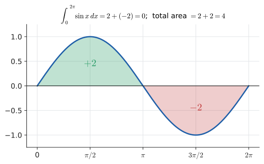
This is the right behaviour for many applications: if \(v(t)\) is a velocity (which can be negative when you reverse), \(\int v\,dt\) is your net displacement, and driving 5 miles forward then 5 back gives 0.
|
Signed area is not total area
If a question asks for the area of a region (a geometric quantity, always positive) or the total distance travelled, you must split the interval where \(f\) changes sign and add the absolute values of the pieces. \(\int_0^{2\pi}\sin x\,dx = 0\), but the total area between the sine curve and the axis over that interval is \(2 + 2 = 4\). |
19.3.4. Properties
These follow directly from the rectangle picture, and you will use them constantly.
The first two together are called linearity. The last one is a definition that keeps the third rule true in all orders.
|
Why the long S, and why "dx"?
Gottfried Leibniz introduced \(\int\) in a manuscript of 29 October 1675, writing it as a stretched letter long-s, the way "s" was then often written in the middle of words. He thought of \(dx\) as an "infinitely small" difference and of \(\int f\,dx\) as a literal sum of infinitely many infinitely thin rectangles. Mathematicians spent the next two centuries making that idea rigorous (Cauchy, then Riemann, then Lebesgue), but Leibniz’s notation was so well chosen that it survived unchanged and still does much of the thinking for you, as you’ll see with substitution. |
|
Integrable or not?
Every continuous function on a closed interval is integrable, and so is any function with finitely many jumps. A function that is not Riemann-integrable is the Dirichlet function: 1 on rational numbers, 0 on irrationals. Every subinterval contains both kinds of number, so you can make any Riemann sum equal 0 or \(b - a\) just by choosing the sample points. Henri Lebesgue’s 1902 theory of integration handles it (the answer is 0) and underpins modern probability. |
19.4. The Fundamental Theorem of Calculus
19.4.1. The problem
Computing \(\int_0^2 x^2\,dx\) from the limit took a special summation formula and some algebra. For \(\int_0^\pi \sin x\,dx\) the same route is miserable. We need a shortcut, and there is a spectacular one.
19.4.2. Intuition: the rate at which area grows
Fix a starting point \(a\) and let the right-hand end vary. Define the accumulation function
the area under \(f\) from \(a\) up to \(x\). (We use \(t\) inside so that \(x\) can be the moving endpoint; the dummy variable’s name does not matter.)
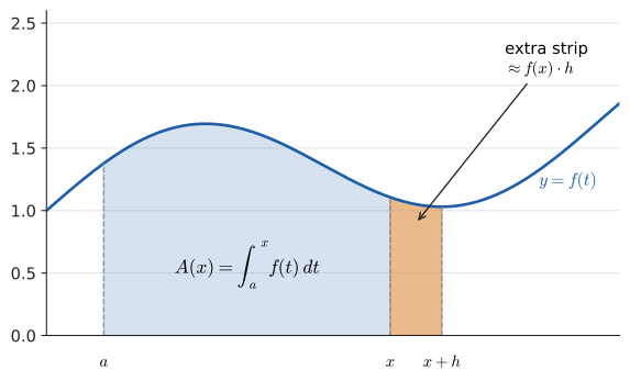
Ask a derivative question about it: how fast does \(A\) grow as \(x\) moves right? Picture yourself painting the region under the curve with a roller moving left to right. The rate at which paint goes on is the height of the strip under the roller right now. Tall curve, area grows quickly; curve near zero, area barely grows; curve negative, the signed area shrinks.
19.4.3. Why it works
Move the endpoint from \(x\) to \(x + h\). The extra area is a thin strip of width \(h\) and height about \(f(x)\):
Divide by \(h\):
The left side is the difference quotient from Chapter 17. As \(h \to 0\) the strip gets thinner, the top of the strip flattens out (because \(f\) is continuous, its height across the strip approaches \(f(x)\)), and the approximation becomes exact. So
To make the "approximately" honest: on the strip, \(f\) lies between its minimum \(m_h\) and maximum \(M_h\), so the strip’s area lies between \(m_h h\) and \(M_h h\), and the difference quotient lies between \(m_h\) and \(M_h\). Continuity forces both to approach \(f(x)\) as \(h \to 0\), so the quotient is squeezed to \(f(x)\).
|
Fundamental Theorem of Calculus, Part 1
If \(f\) is continuous on \({[a, b]}\) and \(A(x) = \int_a^x f(t)\,dt\), then \(A\) is differentiable and
\[\frac{d}{dx}\int_a^x f(t)\,dt = f(x).\]
In words: the rate of change of accumulated area is the current height. Differentiation undoes integration. |
19.4.4. From Part 1 to a computing shortcut
Part 1 says \(A\) is a function whose derivative is \(f\). Any such function is called an antiderivative of \(f\).
|
Antiderivative
An antiderivative of \(f\) is a function \(F\) with \(F'(x) = f(x)\). For example, \(F(x) = x^3/3\) is an antiderivative of \(f(x) = x^2\), because \(\frac{d}{dx}(x^3/3) = x^2\). So is \(x^3/3 + 7\): antiderivatives are only determined up to an added constant. |
Suppose you have found some antiderivative \(F\) of \(f\) by any means, perhaps by recognising a derivative backwards. Both \(F\) and \(A\) have derivative \(f\), so their difference has derivative zero, and a function with zero derivative everywhere on an interval is constant (its graph has slope 0 everywhere, so it is flat). Hence
Find \(C\) by putting \(x = a\): the area from \(a\) to \(a\) is zero, so \(0 = A(a) = F(a) + C\), giving \(C = -F(a)\). Therefore \(A(x) = F(x) - F(a)\), and at \(x = b\):
|
Fundamental Theorem of Calculus, Part 2 (the evaluation theorem)
If \(f\) is continuous on \({[a,b]}\) and \(F\) is any antiderivative of \(f\), then
\[\int_a^b f(x)\,dx = F(b) - F(a) = \Big[\,F(x)\,\Big]_a^b .\]
The bracket notation \(\big[F(x)\big]_a^b\) (also written \(F(x)\big|_a^b\)) means "evaluate at the top limit, minus evaluate at the bottom limit". |
This is astonishing when you first take it in. An infinite limit of sums (an area) is computed by evaluating some other function at two points. All the detail of the curve in between is already encoded in \(F\).
19.4.5. Worked examples
Example 1: the parabola again. An antiderivative of \(x^2\) is \(x^3/3\). Try it: Integrate x² from 0 to 2.
One line, versus the page of summation algebra earlier, and the same answer.
Example 2: one arch of the sine curve. Since \(\frac{d}{dx}(-\cos x) = \sin x\), an antiderivative of \(\sin x\) is \(-\cos x\). Try it: Paint one arch of sin.
The area under one arch of the sine wave is exactly 2. Nothing about the curve suggested a whole number; the theorem delivers it effortlessly.
Example 3: the car. Back to \(v(t) = 20t(3-t) + 10 = -20t^2 + 60t + 10\). Find an antiderivative term by term (each term: raise the power by one, divide by the new power, which we justify properly in the next section): Try it: The car: 120 miles.
Check by differentiating: \(S'(t) = -20t^2 + 60t + 10 = v(t)\). Good. Now evaluate:
The opening question is answered: the car travelled 120 miles. And notice what \(S(t)\) is: a position function, the distance travelled by time \(t\). The FTC is the formal statement that "integrating speed gives distance" and "differentiating distance gives speed" are inverse operations.
|
The car’s speed is not 40 mph, but its average is
120 miles in 3 hours is an average speed of 40 mph. That number has a precise integral meaning (the average value of a function, Section 19.10), and the Mean Value Theorem for integrals guarantees the car was going exactly 40 mph at some instant. Here it happens twice, where \(-20t^2 + 60t + 10 = 40\), at \(t = 1.5 \pm \sqrt{0.75}\), about \(t \approx 0.63\) and \(t \approx 2.37\) hours. |
19.4.6. Part 1 in action
Part 1 is not only theory. It lets you differentiate functions defined by integrals, even when the integral has no formula:
If the upper limit is a function of \(x\), combine with the chain rule. With \(G(u) = \int_0^u \cos(t^2)\,dt\) and upper limit \(u = x^3\):
19.4.7. Where you’d use this
-
Navigation: why phones still need GPS. A phone or drone can track its motion by integrating its accelerometer: velocity is the integral of acceleration, position the integral of velocity (this is inertial navigation). But integration accumulates errors too. A tiny constant sensor bias of \(0.01\) m/s² integrates to a velocity error of \(0.01t\) and a position error of \(\int_0^t 0.01s\,ds = 0.005t^2\) metres: 18 m after one minute, 1.8 km after ten. That quadratic growth is why inertial systems are constantly corrected by GPS or other fixes.
-
Statistics. The probability that a normally distributed quantity is below \(x\) is an integral of the bell curve with a variable upper limit, exactly the \(\int_0^x e^{-t^2}\,dt\) kind of function above. FTC Part 1 says its derivative is the bell curve itself, which is how statistical software moves between a distribution’s cumulative distribution function and its density (Chapter 30).
-
Engineering. The charge on a capacitor is the integral of the current that has flowed into it; the energy stored in a battery is the integral of charging power. Battery-management chips in phones and electric cars run this integral continuously ("coulomb counting") to show you the percentage remaining.
|
Rate in, total out
The FTC needs \(f\) continuous on the whole interval \({[a,b]}\). Applying \(F(b) - F(a)\) across a point where \(f\) blows up gives nonsense. A classic trap is \(\int_{-1}^{1} \frac{1}{x^2}\,dx\). Blindly, \(\big[-1/x\big]_{-1}^{1} = -1 - 1 = -2\), a negative area for a function that is positive everywhere. The real story is that the integral is infinite. See Section 19.11. |
|
Who discovered it?
Isaac Barrow, Newton’s teacher at Cambridge, proved a geometric version of the FTC in 1670. Newton (from the mid-1660s, in his "method of fluxions") and Leibniz (from 1675) each turned it into a general calculus, a mechanical method for computing areas and rates. Their followers spent decades in a bitter priority dispute. Today both are credited with independently inventing calculus, and it is Leibniz’s notation that we use. |
|
Painting the area
Show a curve \(y = f(t)\) on top and, underneath, the graph of the accumulation function \(A(x) = \int_a^x f(t)\,dt\). Drag the endpoint \(x\) and watch the shaded area and \(A(x)\) update together. Show the tangent slope of \(A\) at \(x\) next to the height \(f(x)\): they always match. Try a curve that dips below the axis and watch \(A\) decrease there. |
19.5. Antiderivatives and the constant of integration
19.5.1. The problem
The FTC turns every definite integral into a search: find a function whose derivative is the integrand. So we need a toolkit for running derivative rules in reverse.
19.5.2. Indefinite integrals and \(+C\)
|
Indefinite integral
The indefinite integral \(\int f(x)\,dx\) (no limits) denotes the family of all antiderivatives of \(f\):
\[\int f(x)\,dx = F(x) + C, \qquad \text{where } F'(x) = f(x).\]
\(C\) is the constant of integration: an arbitrary constant, because adding a constant does not change a derivative. A definite integral is a number; an indefinite integral is a family of functions. |
Why must \(+C\) be there? Because \(x^2\), \(x^2 + 1\) and \(x^2 - 5\) all have derivative \(2x\). Graphically, they are vertical shifts of the same curve and have identical slopes at every \(x\). Knowing only the slope, you cannot know the height. For a car: knowing your speed at every moment tells you how far you went, but not where you started. To pin down \(C\) you need one extra fact, an initial condition such as "at \(t = 0\) the car was at mile marker 40".
In a definite integral \(C\) always cancels, \((F(b) + C) - (F(a) + C) = F(b) - F(a)\), which is why we drop it there.
19.5.3. Basic rules: derivative rules run backwards
Each entry is a derivative fact read from right to left. You can check any of them by differentiating the right-hand side.
| Integrand \(f(x)\) | Antiderivative \(\int f(x)\,dx\) | Check: derivative of the answer |
|---|---|---|
\(x^n\) (\(n \ne -1\)) |
\(\dfrac{x^{n+1}}{n+1} + C\) |
\(\frac{(n+1)x^n}{n+1} = x^n\) |
\(\dfrac{1}{x}\) |
\(\ln\lvert x\rvert + C\) |
\(\frac{1}{x}\) (for \(x>0\) and \(x<0\)) |
\(e^x\) |
\(e^x + C\) |
\(e^x\) |
\(e^{kx}\) |
\(\dfrac{1}{k}e^{kx} + C\) |
\(\frac{1}{k}\cdot k e^{kx}\) (chain rule) |
\(\sin x\) |
\(-\cos x + C\) |
\(-(-\sin x)\) |
\(\cos x\) |
\(\sin x + C\) |
\(\cos x\) |
\(\sec^2 x\) |
\(\tan x + C\) |
\(\sec^2 x\) |
\(\dfrac{1}{1+x^2}\) |
\(\arctan x + C\) |
\(\frac{1}{1+x^2}\) |
\(a^x\) |
\(\dfrac{a^x}{\ln a} + C\) |
\(\frac{a^x \ln a}{\ln a}\) |
And the linearity rules carry over from derivatives: \(\int (f + g)\,dx = \int f\,dx + \int g\,dx\) and \(\int c f\,dx = c\int f\,dx\).
Input: an integral \(\int_a^b f(x)\,dx\) with \(f\) continuous on \({[a,b]}\).
Steps:
-
Rewrite the integrand as a sum of standard forms (expand brackets, write roots as powers, split fractions).
-
Find an antiderivative \(F\) term by term using the table and linearity.
-
Check by differentiating \(F\): you must get \(f\) back.
-
Compute \(F(b)\) and \(F(a)\) separately, with brackets around each.
-
Subtract: \(F(b) - F(a)\).
Output: the exact value of the integral.
19.5.4. Worked examples
Example 1. Evaluate \(\int_1^3 (3x^2 - 4x + 5)\,dx\). Try it: Evaluate this integral.
Example 2. Find \(\displaystyle\int \Bigl(2\sqrt{x} - \frac{3}{x} + e^{2x}\Bigr)\,dx\).
First rewrite \(\sqrt{x} = x^{1/2}\). Then
Check: \(\frac{d}{dx}\bigl(\frac43 x^{3/2}\bigr) = \frac43\cdot\frac32 x^{1/2} = 2\sqrt{x}\); the other two terms differentiate back correctly too.
Example 3: using an initial condition. A function satisfies \(f'(x) = 6x - 2\) and \(f(1) = 5\). Find \(f\).
19.5.5. Mechanics: where the "suvat" equations come from
If you did UK Mechanics you memorised the constant-acceleration equations. They are just two integrations. Let acceleration be the constant \(a\), with initial velocity \(u\) and initial position 0 (the old notation used \(s\) for displacement and \(v\) for velocity).
Velocity is the antiderivative of acceleration:
Displacement is the antiderivative of velocity:
A ball thrown straight up at \(u = 20\text{ m/s}\) with \(a = -9.8\text{ m/s}^2\) has \(v(2) = 20 - 19.6 = 0.4\) m/s and \(s(2) = 40 - 19.6 = 20.4\) m. We will reproduce those numbers numerically in Section 19.13. The area under the velocity–time graph is the displacement, exactly as the Mechanics syllabus said, and now you know why.
|
Common antiderivative mistakes
|
|
Differentiation is mechanical, integration is an art
Every combination of elementary functions has an elementary derivative, found mechanically by the rules. Integration is different: many innocent-looking functions have no antiderivative expressible with elementary functions. \(e^{-x^2}\), \(\sin(x)/x\), \(\sqrt{1 + x^3}\) and \(\cos(x^2)\) are examples. Their integrals still exist as numbers (areas), so we either give them new names (\(e^{-x^2}\) leads to the error function \(\operatorname{erf}\), essential in statistics) or compute them numerically. Liouville in the 1830s proved such results, and the Risch algorithm (1969), used in computer algebra systems, decides whether an elementary antiderivative exists. |
19.6. Exercises: Riemann sums, the definite integral and the FTC
-
Recognition. In \(\int_{-1}^{4}(t^3 + 1)\,dt\), name the integrand, the limits of integration and the variable of integration. Is the result a number or a function?
-
Recognition. Without calculating, explain why \(\int_{-1}^{1} x^3\,dx = 0\).
-
Application. For \(f(x) = x^3\) on \({[0,2]}\) with \(n = 4\), compute the left, right and midpoint sums. Compare with the exact value.
-
Application. Use geometry (not antiderivatives) to evaluate \(\int_{-2}^{2}\sqrt{4 - x^2}\,dx\) and \(\int_0^3 (2x - 2)\,dx\).
-
Application. Evaluate \(\int_0^1 (x^4 - 2x + 3)\,dx\), \(\int_1^e \frac{1}{x}\,dx\) and \(\int_0^{\pi/2}\cos x\,dx\).
-
Application. Find \(\frac{d}{dx}\int_0^x \cos(t^2)\,dt\) and \(\frac{d}{dx}\int_1^{x^2}\frac{\sin t}{t}\,dt\).
-
Problem solving. A particle has acceleration \(a(t) = 6t\) m/s², initial velocity 2 m/s and initial position 1 m. Find its position at \(t = 2\).
Answers
-
Integrand \(t^3 + 1\); lower limit \(-1\), upper limit 4; variable \(t\). The result is a number.
-
\(x^3\) is an odd function: \((-x)^3 = -x^3\). The area from \(-1\) to 0 is a mirror image (below the axis) of the area from 0 to 1 (above), so the signed areas cancel.
-
\(\Delta x = 0.5\). Left: \(0.5(0 + 0.125 + 1 + 3.375) = 2.25\). Right: \(0.5(0.125 + 1 + 3.375 + 8) = 6.25\). Midpoint: \(0.5(0.015625 + 0.421875 + 1.953125 + 5.359375) = 0.5 \times 7.75 = 3.875\). Exact: \(\big[x^4/4\big]_0^2 = 4\). The midpoint sum is closest.
-
\(y = \sqrt{4 - x^2}\) is the top half of a circle of radius 2, so the area is \(\tfrac12\pi\cdot 2^2 = 2\pi\). For \(2x - 2\): from 0 to 1 it is below the axis, a triangle of area \(\tfrac12\cdot1\cdot2 = 1\), counted as \(-1\); from 1 to 3 it is a triangle of area \(\tfrac12\cdot 2\cdot 4 = 4\). Total signed area \(4 - 1 = 3\). (Check: \(\big[x^2 - 2x\big]_0^3 = 9 - 6 = 3\).)
-
\(\big[x^5/5 - x^2 + 3x\big]_0^1 = 0.2 - 1 + 3 = 2.2\). \(\big[\ln x\big]_1^e = 1 - 0 = 1\). \(\big[\sin x\big]_0^{\pi/2} = 1 - 0 = 1\).
-
By FTC Part 1, the first is \(\cos(x^2)\). For the second, with upper limit \(u = x^2\): \(\frac{\sin(x^2)}{x^2}\cdot 2x = \frac{2\sin(x^2)}{x}\).
-
\(v(t) = 3t^2 + C_1\), \(v(0) = 2\) gives \(v = 3t^2 + 2\). \(s(t) = t^3 + 2t + C_2\), \(s(0) = 1\) gives \(s = t^3 + 2t + 1\). So \(s(2) = 8 + 4 + 1 = 13\) m.
19.7. Substitution: the chain rule in reverse
19.7.1. The problem
What is \(\int 2x\cos(x^2)\,dx\)? It is not in the table, and it is a product, so linearity does not help. But stare at it: \(x^2\) sits inside the cosine, and \(2x\), the derivative of \(x^2\), sits outside. That pattern is the fingerprint of the chain rule.
19.7.2. Why it works
The chain rule (Chapter 17) says
Read it backwards: if an integrand has the form \(f(g(x))\,g'(x)\) and \(F\) is an antiderivative of \(f\), then
Leibniz notation makes this almost automatic. Name the inner function \(u = g(x)\). Then \(\frac{du}{dx} = g'(x)\), which we write as the differential statement \(du = g'(x)\,dx\). The integrand’s \(g'(x)\,dx\) becomes \(du\) and the inner function becomes \(u\):
|
u-substitution
Substitution (or u-substitution, or change of variables) rewrites an integral in terms of a new variable \(u = g(x)\), replacing \(g'(x)\,dx\) by \(du\). It is the chain rule run backwards. It works when the integrand contains an inner function and (up to a constant factor) that inner function’s derivative. |
Input: an integral \(\int h(x)\,dx\) (or \(\int_a^b h(x)\,dx\)).
Steps:
-
Spot an inner function \(u = g(x)\) whose derivative \(g'(x)\) also appears as a factor (a constant multiple is fine).
-
Compute \(du = g'(x)\,dx\) and solve for whatever piece of the integrand you need, e.g. \(x\,dx = \tfrac12 du\).
-
Rewrite the entire integrand in terms of \(u\) and \(du\). No \(x\) may remain; if it does, choose a different \(u\) or a different method.
-
For a definite integral, convert the limits too: \(x = a \mapsto u = g(a)\) and \(x = b \mapsto u = g(b)\).
-
Integrate in \(u\).
-
Indefinite: substitute \(u = g(x)\) back and add \(C\). Definite: evaluate at the new limits (no back-substitution needed).
Output: the antiderivative or the value of the integral. Check an antiderivative by differentiating.
19.7.3. Worked examples
Example 1. \(\int 2x\cos(x^2)\,dx\). Try it: See u = x² stretch strips; Integrate 2x cos(x²).
Check: \(\frac{d}{dx}\sin(x^2) = \cos(x^2)\cdot 2x\). Correct.
Example 2: a missing constant. \(\int \frac{x}{x^2 + 1}\,dx\). Try it: Integrate x/(x² + 1).
Example 3: a definite integral with changed limits. \(\int_0^1 x(x^2 + 1)^3\,dx\). Try it: Substitution strips for Example 3; Evaluate this integral.
Alternative approach for Example 3. You could also find the indefinite integral \(\tfrac18(x^2+1)^4 + C\), back-substitute, and evaluate with the original limits: \(\tfrac18(2^4) - \tfrac18(1^4) = \tfrac{15}{8}\). Same answer. Converting the limits is usually less work and avoids one source of error; back-substituting is handy when you want the antiderivative anyway. A third alternative, expanding \((x^2+1)^3\) into a polynomial, works here but becomes hopeless for \((x^2+1)^{20}\) and impossible for \((x^2+1)^{1/2}\).
|
Substitution pitfalls
|
19.8. Integration by parts: the product rule in reverse
19.8.1. The problem
Substitution handles "function of a function times the inner derivative". It cannot do \(\int x e^x\,dx\): there is no inner function whose derivative is lying around. This is a product of two unrelated kinds of function, a polynomial and an exponential, and its reverse partner is the product rule.
19.8.2. Why it works
The product rule says \((uv)' = u'v + uv'\). Integrate both sides:
Rearrange to isolate one of the integrals:
In differential shorthand, with \(du = u'\,dx\) and \(dv = v'\,dx\):
The formula trades one integral for another. It helps when the new integral \(\int v\,du\) is easier than the original. The trick is to choose \(u\) as the factor that gets simpler when differentiated (\(x \to 1\), \(\ln x \to 1/x\)) and \(dv\) as the factor you can easily integrate without it getting worse (\(e^x\), \(\sin x\)).
|
Integration by parts
Integration by parts is the formula \(\int u\,dv = uv - \int v\,du\), obtained by integrating the product rule. For definite integrals: \(\int_a^b u\,dv = \big[uv\big]_a^b - \int_a^b v\,du\). A rough guide for choosing \(u\) is LIATE: Logarithmic, Inverse trig, Algebraic (powers of \(x\)), Trigonometric, Exponential, taking as \(u\) whichever comes first in that list. |
Input: an integral \(\int f(x)\,g(x)\,dx\) of a product.
Steps:
-
Choose \(u\) (the factor that simplifies when differentiated; use LIATE) and let \(dv\) be everything else, including \(dx\).
-
Compute \(du = u'\,dx\) by differentiating, and \(v\) by integrating \(dv\) (no \(+C\) needed here).
-
Write \(uv - \int v\,du\).
-
Evaluate the new integral. If it is no easier, go back and swap the choices.
-
Add \(+C\) (indefinite) or evaluate between limits (definite).
Output: the antiderivative or value. Check by differentiating.
19.8.3. Worked examples
Example 1. \(\int x e^x\,dx\). Algebraic beats exponential in LIATE, so \(u = x\). Try it: Integrate x eˣ.
Check: \(\frac{d}{dx}\bigl(e^x(x-1)\bigr) = e^x(x - 1) + e^x\cdot 1 = x e^x\). Correct.
What if we had chosen the other way, \(u = e^x\), \(dv = x\,dx\)? Then \(v = x^2/2\) and the new integral is \(\int \frac{x^2}{2}e^x\,dx\), which is worse. That is the signal to swap.
Example 2: the "invisible" second factor. \(\int \ln x\,dx\). There seems to be only one factor, but write it as \(\ln x \cdot 1\). Try it: Integrate ln x.
Example 3: a definite integral. \(\int_0^{\pi} x\sin x\,dx\).
Example 4: going round in a circle on purpose. \(I = \int e^x\sin x\,dx\). Parts twice, with \(u\) the trig factor both times:
The original integral \(I\) has reappeared. Treat it as an unknown and solve: \(2I = e^x(\sin x - \cos x)\), so
Where you’d use this. Integration by parts is how averages of "\(x\) times a density" are computed. If the waiting time for the next request at a server has the exponential density \(\lambda e^{-\lambda x}\) (see Section 19.10), the mean wait is \(\int_0^\infty x\,\lambda e^{-\lambda x}\,dx\). Parts with \(u = x\), \(dv = \lambda e^{-\lambda x}dx\) gives \(\bigl[-xe^{-\lambda x}\bigr]_0^\infty + \int_0^\infty e^{-\lambda x}\,dx = 0 + \frac{1}{\lambda}\): at \(\lambda = 0.5\) requests per second, the average wait is 2 seconds. The same calculation gives the mean lifetime of a radioactive nucleus and the expected time to failure of a component in reliability engineering. Substitution, meanwhile, is how the normal distribution is standardised: \(z = (x - \mu)/\sigma\) turns every bell-curve integral into one with \(\mu = 0\), \(\sigma = 1\), which is why a single \(z\)-table (or one library function) serves them all.
19.8.4. Choosing a method
| What you see | Method | Example |
|---|---|---|
A sum of standard forms |
Table + linearity |
\(\int (x^3 - 4\cos x)\,dx\) |
An inner function and its derivative (up to a constant) |
Substitution |
\(\int x^2 e^{x^3}\,dx\) |
A product of two different kinds of function, one of which simplifies when differentiated |
Parts |
\(\int x^2\cos x\,dx\) (parts twice) |
A single \(\ln\) or inverse-trig function |
Parts with \(dv = dx\) |
\(\int \arctan x\,dx\) |
A rational function \(p(x)/q(x)\) |
Algebra first (division, partial fractions) |
\(\int \frac{1}{x^2 - 1}\,dx\) |
No elementary antiderivative, or only data points |
Numerical integration |
\(\int_0^1 e^{-x^2}\,dx\) |
Try it: Partial fractions of 1/(x² − 1).
In practice, professionals reach for a computer algebra system (SymPy, Mathematica) for hard symbolic integrals, and for numerical methods whenever only a number is needed. The point of learning substitution and parts is not to compete with software; it is to read the formulas in papers and textbooks (many derivations are a substitution or parts step in disguise) and to be able to check what software tells you.
|
Partial fractions, trig substitution and the rest
A traditional calculus course spends weeks on further techniques: partial fractions, trigonometric substitution, reduction formulas, tables of hundreds of integrals. The Victorian Cambridge "Tripos" examinations made integration a competitive sport. Today these are worth recognising, not drilling. Richard Feynman famously preferred another trick, "differentiating under the integral sign", which he learned from an old textbook and which let him solve integrals that stumped his colleagues at Los Alamos. |
|
Watching a substitution
Plot \(2x\cos(x^2)\) on \({[0, \sqrt{\pi}]}\) beside \(\cos u\) on \({[0, \pi]}\), with a slider that moves a thin strip in one plot and the corresponding strip in the other. The strips have different widths and heights but the same area: substitution is a stretching of the horizontal axis that preserves area. Try it: Open the substitution lab |
19.9. Exercises: techniques of integration
-
Recognition. For each, say which method you would use and why: (a) \(\int x^2 e^x\,dx\), (b) \(\int x^2 e^{x^3}\,dx\), (c) \(\int (e^x + x^2)\,dx\).
-
Application. \(\int 3x^2(x^3 + 1)^5\,dx\).
-
Application. \(\int \cos x\,e^{\sin x}\,dx\).
-
Application. \(\int_0^1 x e^{x^2}\,dx\).
-
Application. \(\int x\cos x\,dx\).
-
Problem solving. \(\int_1^e x\ln x\,dx\).
-
Problem solving. \(\int x^2 e^x\,dx\) (parts twice).
Answers
-
(a) Parts: product of a polynomial and an exponential, with no inner-function pattern; \(u = x^2\), twice. (b) Substitution: \(u = x^3\) and \(du = 3x^2\,dx\) is present up to a factor \(\tfrac13\). (c) Table and linearity: \(e^x + x^3/3 + C\).
-
\(u = x^3 + 1\), \(du = 3x^2\,dx\): \(\int u^5\,du = u^6/6 + C = (x^3+1)^6/6 + C\).
-
\(u = \sin x\), \(du = \cos x\,dx\): \(\int e^u\,du = e^{\sin x} + C\).
-
\(u = x^2\), \(x\,dx = \tfrac12 du\), limits 0 to 1: \(\tfrac12\int_0^1 e^u\,du = \tfrac12(e - 1) \approx 0.8591\).
-
\(u = x\), \(dv = \cos x\,dx\), \(v = \sin x\): \(x\sin x - \int\sin x\,dx = x\sin x + \cos x + C\).
-
\(u = \ln x\) (L before A), \(dv = x\,dx\), \(du = dx/x\), \(v = x^2/2\). \(\big[\tfrac{x^2}{2}\ln x\big]_1^e - \int_1^e \tfrac{x}{2}\,dx = \tfrac{e^2}{2} - \big[\tfrac{x^2}{4}\big]_1^e = \tfrac{e^2}{2} - \tfrac{e^2}{4} + \tfrac14 = \tfrac{e^2 + 1}{4} \approx 2.0973\).
-
\(u = x^2\), \(v = e^x\): \(x^2e^x - \int 2x e^x\,dx\). Then by Example 1, \(\int 2xe^x\,dx = 2e^x(x - 1)\). Total: \(e^x(x^2 - 2x + 2) + C\). Check: derivative is \(e^x(x^2 - 2x + 2) + e^x(2x - 2) = x^2 e^x\).
19.10. Applications: slice, approximate, sum, integrate
Almost every application of integration follows one pattern, and it is worth stating explicitly because it is how you set up integrals for problems no textbook has seen.
Input: a quantity \(Q\) that is a total of something varying along a variable \(x\) from \(a\) to \(b\).
Steps:
-
Slice: cut the range \({[a,b]}\) into thin pieces of width \(\Delta x\).
-
Approximate: on one slice at position \(x\), treat everything as constant and write the slice’s contribution as \(\Delta Q \approx (\text{something in } x)\times\Delta x\).
-
Sum: the total is approximately the Riemann sum of those contributions.
-
Integrate: let \(\Delta x \to 0\), replacing the sum by \(\int_a^b (\text{something in } x)\,dx\).
-
Evaluate (FTC, or numerically).
Output: \(Q\) as a definite integral, and its value.
19.10.1. Area between curves
Problem. Find the area enclosed between \(y = x\) and \(y = x^2\). Try it: Area between x and x².
Slice and approximate. The curves meet where \(x = x^2\), that is \(x(x - 1) = 0\), so at \(x = 0\) and \(x = 1\). Between them, \(x > x^2\) (try \(x = 0.5\): \(0.5 > 0.25\)), so a thin vertical slice at position \(x\) has height \(\text{top} - \text{bottom} = x - x^2\) and area \((x - x^2)\,\Delta x\).
Integrate.
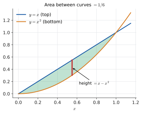
In general, \(\text{Area} = \int_a^b \bigl(\text{top}(x) - \text{bottom}(x)\bigr)\,dx\). Because we subtract heights, it does not matter whether the curves are above or below the axis. If the curves cross inside the interval, split at the crossings so that "top" really is on top in each piece.
19.10.2. Average value of a function
The average of \(n\) numbers is their sum divided by \(n\). For a function, sample it at \(n\) evenly spaced points and average:
The right side is a Riemann sum divided by \(b - a\). Letting \(n \to \infty\):
|
Average value
The average value of \(f\) on \({[a,b]}\) is
\[\bar f = \frac{1}{b - a}\int_a^b f(x)\,dx.\]
Geometrically, it is the height of the rectangle on \({[a,b]}\) with the same area as the region under \(f\). |
Example. The average value of \(\sin x\) over one arch \({[0, \pi]}\) is \(\frac{1}{\pi}\cdot 2 = \frac{2}{\pi} \approx 0.6366\). Electrical engineers use exactly this (and the related root-mean-square average) to relate peak and average AC voltages. The car’s average speed was \(\tfrac13\cdot 120 = 40\) mph.
19.10.3. Volumes of revolution (briefly)
Spin the curve \(y = f(x)\), \(a \le x \le b\), around the \(x\)-axis. The solid it sweeps out can be sliced like a salami into thin discs. The slice at \(x\) is a cylinder of radius \(f(x)\) and thickness \(\Delta x\), with volume \(\pi f(x)^2\,\Delta x\). Sum and integrate (the disc method): Try it: Spin a semicircle into a sphere.
Example: a sphere. The upper half of a circle of radius \(r\) is \(y = \sqrt{r^2 - x^2}\) for \(-r \le x \le r\). Spinning it gives a sphere:
The school formula for the volume of a sphere, which you probably memorised without proof, falls straight out.
19.10.4. Work
In physics, the work done by a constant force \(F\) moving an object a distance \(d\) in the direction of the force is \(W = Fd\) (in joules when \(F\) is in newtons and \(d\) in metres). When the force varies with position, slice:
Example: stretching a spring. Hooke’s law says a spring stretched by \(x\) metres pulls back with force \(F = kx\). For \(k = 200\) N/m, the work to stretch it 0.1 m from rest is
Example: winding up a hanging chain. A 10 m chain of mass 2 kg/m hangs from a winch. The slice of chain at depth \(y\) (thickness \(\Delta y\)) weighs \(2 \times 9.8\,\Delta y\) newtons and must be lifted \(y\) metres, so it needs work \(19.6\,y\,\Delta y\). Total:
Here the force is constant but the distance varies by slice, a different variation from the spring. The slice method does not care which.
19.10.5. Probability densities
For a continuous random quantity, such as the waiting time until the next request hits a server, it makes no sense to ask for the probability of exactly 1.000000 seconds. Instead a probability density function \(p(x)\) describes how probability is spread out, and probabilities are areas:
Example. Waiting times are often modelled by the exponential density \(p(x) = \lambda e^{-\lambda x}\) for \(x \ge 0\). With \(\lambda = 0.5\) per second, the probability of waiting at most 1 second is
The integral of the density over \({[0, \infty)}\) is \(1\), an improper integral (next section). The whole of Chapter 30 is built on this idea, including the normal (bell) curve, whose integral is the famous non-elementary \(\int e^{-x^2}\,dx\).
19.10.6. Accumulated quantities and net change
The car example generalises: the integral of a rate of change gives the total change. If \(Q'(t)\) is a rate,
This is FTC Part 2 read physically, and it is sometimes called the net change theorem. Water flowing into a tank at \(r(t) = 10 + 2t\) litres per minute adds \(\int_0^5 (10 + 2t)\,dt = \big[10t + t^2\big]_0^5 = 50 + 25 = 75\) litres in the first 5 minutes. The same pattern turns power (watts) into energy (joules or kWh), a bandwidth curve (bytes per second) into total data transferred, and a births-minus-deaths rate into a population change.
|
Setting up integrals
|
19.11. Improper integrals: infinite regions with finite area
19.11.1. The problem
Can a region that stretches out to infinity have finite area? Our definition used a closed interval \({[a,b]}\), so we need to extend it. And we need to, because probability densities live on unbounded intervals.
19.11.2. The method: take a limit
Integrate up to a finite cut-off \(b\), then let \(b \to \infty\):
If the limit exists and is finite, the integral converges; otherwise it diverges.
|
Improper integral
An improper integral is one where the interval is unbounded (a limit of integration is \(\pm\infty\)) or the integrand blows up somewhere in the interval. It is defined as a limit of ordinary integrals and is said to converge if that limit is a finite number and diverge otherwise. |
19.11.3. Two worked examples that look alike but are not
Example 1: \(\int_1^\infty \frac{1}{x^2}\,dx\). Try it: ∫ 1/x² to infinity; ∫ 1/x to infinity.
It converges: the infinitely long region has area exactly 1.
Example 2: \(\int_1^\infty \frac{1}{x}\,dx\).
It diverges. Both curves fall to zero, and \(1/x\) is only a little larger than \(1/x^2\) far out, but \(1/x\) doesn’t fall fast enough: the area keeps growing (slowly, like a logarithm) forever.
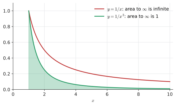
The general rule (the p-test): \(\int_1^\infty x^{-p}\,dx\) converges exactly when \(p > 1\), with value \(\frac{1}{p - 1}\). The borderline case \(p = 1\) diverges.
Example 3: an integrand that blows up. \(\int_0^1 \frac{1}{\sqrt{x}}\,dx\). The integrand is infinite at \(x = 0\), so cut off at \(c > 0\): Try it: A spike with finite area; Evaluate this improper integral.
A spike to infinity with finite area 2. (For \(\int_0^1 \frac1x\,dx\) the same calculation gives \(-\ln c \to \infty\): divergent.)
|
The fake negative area, revisited
An integrand that blows up inside the interval is improper even though both limits are finite. \(\int_{-1}^1 \frac{1}{x^2}\,dx\) must be split at 0 into two improper integrals, and \(\int_0^1 x^{-2}\,dx = \lim_{c\to0^+}\bigl(\tfrac1c - 1\bigr) = \infty\), so the whole thing diverges. Always scan the interval for vertical asymptotes before applying the FTC. |
|
Gabriel’s horn
Spin \(y = 1/x\) for \(x \ge 1\) around the \(x\)-axis. The volume is \(\pi\int_1^\infty x^{-2}\,dx = \pi\), finite. The surface area turns out to be infinite (it is at least \(2\pi\int_1^\infty \frac1x\,dx\)). So you could fill the horn with \(\pi\) units of paint but never paint its inside surface. Evangelista Torricelli’s 1643 discovery shocked contemporaries who believed infinite objects must have infinite size in every sense. |
Try it: Gabriel’s horn’s volume.
19.12. Numerical integration
19.12.1. The problem
Antiderivatives fail us in three common situations:
-
No elementary antiderivative exists: \(\int_0^1 e^{-x^2}\,dx\), the backbone of the normal distribution.
-
The function is only known as data: speed logged by a GPS once a second, power measured every minute.
-
The function is a black box: the output of a simulation or another program.
In all three we want a number, and the Riemann-sum idea gives it directly. The question is how to get high accuracy from few function evaluations. This is called numerical integration or quadrature.
|
Quadrature
Quadrature means numerical approximation of a definite integral. The name comes from the ancient problem of "squaring" a shape: constructing a square with the same area. A quadrature rule is a weighted sum \(\sum w_i f(x_i)\) of function values at chosen nodes \(x_i\). |
19.12.2. The trapezoid rule
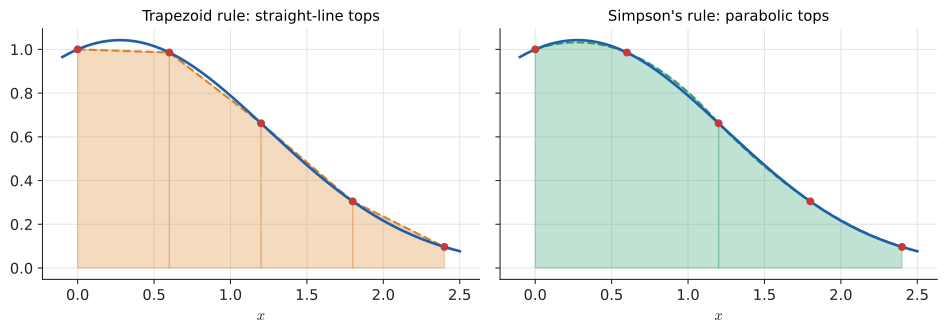
Intuition. Instead of flat-topped rectangles, join neighbouring points on the curve with straight lines. Each strip becomes a trapezoid, which hugs a smooth curve much better than a rectangle.
Why it works. A trapezoid with parallel sides \(f(x_{i-1})\) and \(f(x_i)\) and width \(h\) has area \(\frac{h}{2}\bigl(f(x_{i-1}) + f(x_i)\bigr)\). Add the \(n\) strips. Every interior point is shared by two neighbouring trapezoids, so it is counted twice; the two endpoints are counted once:
It is also exactly the average of the left and right Riemann sums.
19.12.3. Simpson’s rule
Intuition. Straight lines cannot follow curvature. Parabolas can. Take the points in groups of three, fit the unique parabola through each triple, and integrate the parabola exactly.
Why it works. Shift a triple so the middle node is at 0: nodes \(-h, 0, h\) with heights \(y_0, y_1, y_2\). For a parabola \(q(x) = Ax^2 + Bx + C\) through them,
The \(Bx\) term integrates to zero (odd function). From the three points, \(q(0) = C = y_1\) and \(y_0 + y_2 = q(-h) + q(h) = 2Ah^2 + 2C\), so \(2Ah^2 = y_0 + y_2 - 2y_1\). Substitute:
The middle point gets weight 4, the ends weight 1. Chaining pairs of strips across \({[a,b]}\) (so \(n\) must be even) gives weights \(1, 4, 2, 4, 2, \dots, 4, 1\):
Input: \(f\), interval \({[a,b]}\), number of strips \(n\).
Steps:
-
Set \(h = (b - a)/n\) and nodes \(x_i = a + ih\) for \(i = 0,\dots,n\).
-
Evaluate \(f(x_0), \dots, f(x_n)\).
-
Form \(\tfrac12 f(x_0) + f(x_1) + \dots + f(x_{n-1}) + \tfrac12 f(x_n)\).
-
Multiply by \(h\).
Output: \(T_n \approx \int_a^b f(x)\,dx\). Error shrinks like \(h^2\): doubling \(n\) cuts the error by about 4.
Input: \(f\), interval \({[a,b]}\), an even number of strips \(n\).
Steps:
-
Set \(h = (b - a)/n\) and nodes \(x_i = a + ih\).
-
Evaluate \(f\) at every node.
-
Weight the values \(1, 4, 2, 4, \dots, 2, 4, 1\): endpoints 1, odd-indexed nodes 4, interior even-indexed nodes 2.
-
Add the weighted values and multiply by \(h/3\).
Output: \(S_n \approx \int_a^b f(x)\,dx\). Error shrinks like \(h^4\): doubling \(n\) cuts the error by about 16.
19.12.4. Worked example by hand: estimating \(\ln 2\)
We know \(\int_1^2 \frac{1}{x}\,dx = \ln 2 \approx 0.693147\). Pretend we don’t, and use \(n = 4\), \(h = 0.25\). Try it: Trapezoid and Simpson for ln 2.
Nodes and values:
| \(i\) | 0 | 1 | 2 | 3 | 4 |
|---|---|---|---|---|---|
\(x_i\) |
1 |
1.25 |
1.5 |
1.75 |
2 |
\(f(x_i) = 1/x_i\) |
1 |
0.8 |
0.666667 |
0.571429 |
0.5 |
Trapezoid:
Error: \(0.697024 - 0.693147 = 0.003877\).
Simpson:
Error: \(0.693254 - 0.693147 = 0.000107\). The same five function values give a result 36 times more accurate, just by weighting them more cleverly.
19.12.5. Implementation and error comparison
import math

def trapezoid(f, a, b, n):
    h = (b - a) / n
    total = (f(a) + f(b)) / 2
    for i in range(1, n):
        total += f(a + i * h)
    return h * total

def simpson(f, a, b, n):
    if n % 2:
        raise ValueError("Simpson's rule needs an even number of subintervals")
    h = (b - a) / n
    total = f(a) + f(b)
    for i in range(1, n):
        weight = 4 if i % 2 else 2
        total += weight * f(a + i * h)
    return h * total / 3

exact = 2.0   # integral of sin x from 0 to pi
print(" n    trapezoid error   Simpson error")
for n in [2, 4, 8, 16, 32]:
    et = abs(trapezoid(math.sin, 0, math.pi, n) - exact)
    es = abs(simpson(math.sin, 0, math.pi, n) - exact)
    print(f"{n:3d}   {et:.3e}         {es:.3e}")
Try it: Watch the errors shrink.
 n    trapezoid error   Simpson error
  2   4.292e-01         9.440e-02
  4   1.039e-01         4.560e-03
  8   2.577e-02         2.692e-04
 16   6.430e-03         1.659e-05
 32   1.607e-03         1.033e-06
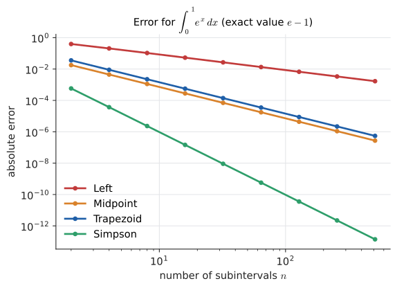
Read the columns as ratios. Each doubling of \(n\) divides the trapezoid error by about 4 (\(0.1039 / 0.02577 \approx 4.03\)) and the Simpson error by about 16 (\(2.692\times10^{-4} / 1.659\times10^{-5} \approx 16.2\)). That is what "error \(\propto h^2\)" and "error \(\propto h^4\)" mean in practice. On a log–log plot those become straight lines of slope \(-2\) and \(-4\); the left Riemann sum has slope \(-1\).
19.12.6. Choosing a method
| Situation | Choose |
|---|---|
Smooth function, can evaluate anywhere, want accuracy cheaply |
Simpson (or library adaptive quadrature such as |
Equally spaced data points, odd number of them |
Simpson |
Data at uneven spacing, or noisy data |
Trapezoid (no smoothness to exploit; simple and robust) |
Periodic function over a whole period |
Trapezoid (it is spectacularly accurate here) |
Integrand with a kink or a jump |
Split at the bad point, then use either rule on each smooth piece |
Many dimensions (say 5 or more) |
Monte Carlo (see the sidebar below) |
An antiderivative is available |
The FTC, exactly |
Try it: The log–log error plot.
Where you’d use this: drug exposure. In clinical trials, blood is sampled at a few times after a dose and the area under the curve (AUC) of concentration measures the body’s total exposure to the drug. With samples at 0, 1, 2, 4 and 8 hours of 0, 8, 10, 6 and 2 mg/L (uneven spacing, so trapezoids), the AUC is \(\tfrac{0 + 8}{2}(1) + \tfrac{8 + 10}{2}(1) + \tfrac{10 + 6}{2}(2) + \tfrac{6 + 2}{2}(4) = 4 + 9 + 16 + 16 = 45\) mg·h/L. Regulators compare generic and brand-name drugs by exactly this number. The same trapezoid rule turns a GPS speed log into the distance on a running app, and a sampled power trace into the energy a server consumed.
|
When numerical integration goes wrong
|
Here is a completely different idea. The integral \(\int_a^b f(x)\,dx\) equals \((b - a)\times\) (the average value of \(f\)). So estimate the average by sampling \(f\) at random points:
import random, math

def monte_carlo(f, a, b, n, seed=2):
    rng = random.Random(seed)
    total = 0.0
    for _ in range(n):
        total += f(rng.uniform(a, b))   # sample a random point, record height
    return (b - a) * total / n          # width times average height

f = lambda x: math.exp(-x * x)
exact = 0.7468241328124271
for n in [100, 10_000, 1_000_000]:
    est = monte_carlo(f, 0, 1, n)
    print(f"n={n:>9,}  estimate={est:.6f}  error={abs(est - exact):.1e}")
n= 100 estimate=0.710943 error=3.6e-02 n= 10,000 estimate=0.748450 error=1.6e-03 n=1,000,000 estimate=0.746796 error=2.8e-05
The error falls roughly like \(1/\sqrt{n}\) (on average; any one run is luckier or unluckier). That is far slower than Simpson in one dimension. So why bother? Because the \(1/\sqrt{n}\) rate does not depend on the dimension. A grid-based rule in 10 dimensions with just 10 points per axis needs \(10^{10}\) evaluations; Monte Carlo doesn’t care. Rendering engines integrate light arriving from all directions at every pixel (path tracing), finance integrates over thousands of random market paths, and Bayesian statistics integrates over many parameters. All use Monte Carlo.
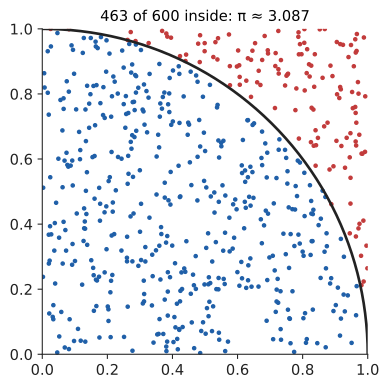
A classic toy version estimates \(\pi\): throw random points into the unit square and count the fraction landing inside the quarter circle, whose area is \(\pi/4\).
|
Gaussian quadrature
Trapezoid and Simpson fix the nodes at equal spacing and choose only the weights. Carl Friedrich Gauss asked in 1814: what if you choose the nodes as well? With \(n\) cleverly placed points (roots of Legendre polynomials) you can integrate every polynomial of degree up to \(2n - 1\) exactly. Two well-chosen points beat Simpson’s three. Variants of Gaussian quadrature sit inside most scientific integration libraries. |
|
Racing the rules
Choose a function from a menu (smooth, kinked, oscillating, spiking) and a number of strips. Show trapezoids, midpoint rectangles and Simpson parabolas overlaid on the curve, with a live log–log error plot growing as you increase \(n\). Find a function where the trapezoid rule beats Simpson (hint: a periodic function over one full period, or one with a kink). Try it: A kink slows Simpson · Race the rules |
19.13. Differential equations: a first look
19.13.1. The problem
So far the rate of change was a known function of time: \(v(t)\) was given, and we integrated to get position. Often, though, the rate depends on the current amount. A population grows faster when there are more organisms. A hot cup of coffee cools faster when it is much hotter than the room. A falling object’s acceleration depends on its velocity through air resistance. Equations relating a quantity to its own rate of change are called differential equations, and they are how science writes down the laws of change.
|
Differential equation
A differential equation is an equation involving an unknown function and its derivatives, such as \(\frac{dy}{dt} = ky\). A solution is a function that makes the equation true. An initial condition such as \(y(0) = y_0\) picks out one solution from the family. An ordinary differential equation (ODE) has a single independent variable (usually time). |
19.13.2. Exponential growth: \(dy/dt = ky\)
Intuition. The rate of growth is proportional to the current size: double the population, double the births per year. You already know a function with that property: \(e^t\) is its own derivative (Chapter 17).
Solving by separation of variables. Move all the \(y\) to one side and all the \(t\) to the other (treating \(dy\) and \(dt\) as Leibniz did, which can be justified by the chain rule), then integrate both sides:
Check: \(\frac{d}{dt}\bigl(y_0 e^{kt}\bigr) = k\,y_0 e^{kt} = ky\). Correct.
Example. Bacteria double every 20 minutes. Then \(e^{20k} = 2\), so \(k = \frac{\ln 2}{20} \approx 0.03466\) per minute. After 2 hours (6 doubling periods) the population is \(e^{120k} = e^{6\ln 2} = 2^6 = 64\) times its initial size. With \(k < 0\) the same equation describes radioactive decay, drug elimination and (via Newton’s law of cooling, \(\frac{dT}{dt} = -k(T - T_{\text{room}})\)) that cooling coffee. See Chapter 12 for more on exponential models.
19.13.3. Newton’s second law is a differential equation
\(F = ma\) says acceleration (the second derivative of position) is force divided by mass:
When \(F\) is constant we integrated twice in Section 19.5 to get the suvat equations. When \(F\) depends on position or velocity (springs, drag, gravity between planets), exact solutions are rare and we must step forward numerically.
19.13.4. Euler’s method: integrating one small step at a time
Intuition. If you know where you are and how fast you are changing right now, assume the rate stays constant for a short time \(\Delta t\) and step forward. Then recompute the rate and repeat. It is a left Riemann sum built on the fly, where each rectangle’s height depends on the result so far.
Input: a rate function \(\frac{dy}{dt} = g(t, y)\), initial values \(t_0, y_0\), a step size \(\Delta t\), and an end time \(T\).
Steps:
-
Set \(t = t_0\), \(y = y_0\).
-
While \(t < T\):
-
Compute the current rate \(r = g(t, y)\).
-
Update \(y \leftarrow y + r\,\Delta t\) (the tangent-line step).
-
Update \(t \leftarrow t + \Delta t\).
-
Output: the approximate values \(y(t)\) at each step. The error at a fixed end time shrinks roughly in proportion to \(\Delta t\).
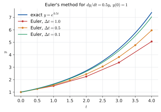
Worked example by hand. \(\frac{dy}{dt} = 0.5y\), \(y(0) = 1\), step \(\Delta t = 1\): Try it: Step through this example.
The exact solution is \(y(4) = e^{2} \approx 7.389\). Each step multiplies by 1.5 instead of \(e^{0.5} \approx 1.6487\), so Euler lags behind because it uses the rate at the start of each step, while the true rate keeps increasing during the step. Smaller steps fix this, as the figure shows.
19.13.5. Mechanics in code: a projectile
For motion we track two quantities, position and velocity, each with its own rate: \(\frac{dy}{dt} = v\) and \(\frac{dv}{dt} = a = F/m\). Try it: Compare the three integrators.
g = 9.8                      # m/s^2, downward
dt = 0.1                     # time step (s)
y, v, t = 0.0, 20.0, 0.0     # height (m), upward velocity (m/s), time (s)
while t < 2.0 - 1e-9:
    a = -g                   # Newton: F = m a  =>  a = F/m = -g
    y = y + v * dt           # position changes at rate v
    v = v + a * dt           # velocity changes at rate a
    t = t + dt
print(f"Euler:  t={t:.1f}  y={y:.3f}  v={v:.3f}")
print(f"Exact:  t=2.0  y={20*2 - 0.5*g*4:.3f}  v={20 - g*2:.3f}")
Euler: t=2.0 y=21.380 v=0.400 Exact: t=2.0 y=20.400 v=0.400
The velocity is exact (its rate is constant, so a left sum is perfect), but the position is off by nearly a metre: each step uses the velocity from the start of the step, which is always a little too high on the way up.
Try it: Euler vs symplectic vs Verlet.
|
A rate that depends on itself
Draw a slope field for \(dy/dt = g(t, y)\): a tiny line segment at each grid point showing the slope there. Click a starting point and watch Euler’s method trace a path through the field with an adjustable \(\Delta t\), alongside the exact solution where known. Try \(dy/dt = 0.5y\), \(dy/dt = -y\), and the logistic equation \(dy/dt = y(1 - y)\). Try it: Open the slope-field lab |
|
Euler on large steps
Euler’s method can be not just inaccurate but unstable. For \(dy/dt = -3y\) with \(\Delta t = 1\), each step multiplies \(y\) by \(1 - 3 = -2\): the "decaying" solution flips sign and doubles every step, exploding instead of decaying. A physics engine with too large a time step on a stiff spring does exactly this, which is why objects sometimes jitter and fly off into space in games. |
Try it: Watch Euler explode.
19.13.6. Where you’d use this
-
Everyday: caffeine. Caffeine is eliminated roughly exponentially, \(\frac{dC}{dt} = -kC\), with a half-life of about 5 hours. A 100 mg coffee at 4 pm leaves \(100\times 2^{-7/5} \approx 38\) mg in your system at 11 pm: more than a third of a cup at bedtime.
-
Epidemiology. The SIR model tracks susceptible, infected and recovered people with three coupled differential equations (for example \(\frac{dI}{dt} = \beta SI - \gamma I\)). Public-health forecasts during the COVID-19 pandemic were refined versions of this, solved by step-by-step methods like Euler’s.
-
Computing. Every physics engine, weather model, circuit simulator (SPICE) and orbital-mechanics program is a differential-equation solver at heart: it knows the rates (forces, currents, winds) and integrates them forward in small time steps, as in the projectile code above.
19.14. Sums and integrals in algorithm analysis
19.14.1. The problem
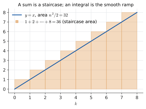
How many times does the inner statement run in this loop? Try it: The loop as a staircase.
count = 0
n = 8
for i in range(1, n + 1):
    for j in range(i):        # inner loop runs i times
        count += 1
print(count)                  # 36
The exact answer is \(\sum_{i=1}^{n} i = \frac{n(n+1)}{2}\), which is 36 for \(n = 8\). For algorithm analysis we usually care about growth: \(\frac{n(n+1)}{2} \approx \frac{n^2}{2}\), so the loop is \(O(n^2)\). Notice that \(\int_0^n x\,dx = \frac{n^2}{2}\) gives the leading term immediately.
19.14.2. Why it works
A sum \(\sum_{k=1}^{n} f(k)\) is a Riemann sum with width 1. If \(f\) is increasing, comparing each unit rectangle with the area under the curve on either side gives the integral bounds
(For decreasing \(f\) the inequalities flip.) The sum is trapped between two integrals that are easy to compute, so it grows at the same rate as the integral.
19.14.3. Worked examples
| Sum | Integral estimate | Where it appears |
|---|---|---|
\(\sum_{k=1}^{n} k\) |
\(\int_0^n x\,dx = \tfrac{n^2}{2}\) |
Nested loops, insertion sort worst case |
\(\sum_{k=1}^{n} k^2\) |
\(\int_0^n x^2\,dx = \tfrac{n^3}{3}\) |
Triple loops over triangles, naive Gaussian elimination |
\(\sum_{k=1}^{n} \tfrac{1}{k}\) |
\(\int_1^n \tfrac{dx}{x} = \ln n\) |
Quicksort, coupon collector, harmonic series |
\(\sum_{k=1}^{n} \ln k = \ln(n!)\) |
\(\int_1^n \ln x\,dx = n\ln n - n + 1\) |
Lower bound \(\Omega(n\log n)\) for comparison sorting |
For the harmonic sum, \(1/x\) is decreasing, so the bounds read \(\ln(n+1) \le H_n \le 1 + \ln n\). For \(n = 1000\) that is \(6.909 \le H_{1000} \le 7.908\); the true value is about \(7.485\). Try it: Bound the harmonic sum.
The last row is worth a moment. \(\int_1^n \ln x\,dx\) uses the integration-by-parts result from Section 19.8, and gives \(\log_2(n!) \approx n\log_2 n\). Since a comparison sort must distinguish all \(n!\) orderings and each comparison gives one bit, no comparison sort can beat roughly \(n\log_2 n\) comparisons. An integration-by-parts exercise proves a fundamental limit of computer science. Try it: ln n! against an integral.
19.15. Exercises: applications, improper integrals and numerics
-
Recognition. Which of these improper integrals converge? \(\int_1^\infty x^{-3}\,dx\), \(\int_1^\infty x^{-1/2}\,dx\), \(\int_0^1 x^{-1}\,dx\).
-
Application. Find the area between \(y = 2x\) and \(y = x^2\). Try it: Area between 2x and x².
-
Application. Find the average value of \(x^2\) on \({[0, 3]}\).
-
Application. Find the volume generated by rotating \(y = x\), \(0 \le x \le 3\), about the \(x\)-axis, and check it against the cone formula \(\tfrac13\pi r^2 h\). Try it: Spin y = x: a cone.
-
Application. Approximate \(\int_0^2 x^3\,dx\) with the trapezoid rule and with Simpson’s rule, both with \(n = 2\). Explain what you notice. Try it: Simpson is exact for cubics.
-
Problem solving. A population of 500 grows according to \(dP/dt = 0.02P\) (time in years). What is it after 50 years? Use Euler’s method with \(\Delta t = 25\) years and compare.
-
Problem solving. Use integral bounds to show that \(\sum_{k=1}^{n} \sqrt{k}\) grows like \(\tfrac23 n^{3/2}\). Try it: Σ√k against ⅔n^(3/2).
Answers
-
\(\int_1^\infty x^{-3}\,dx = \lim_{b\to\infty}\big[-\tfrac{1}{2x^2}\big]_1^b = \tfrac12\): converges (\(p = 3 > 1\)). \(\int_1^\infty x^{-1/2}\,dx = \lim\big[2\sqrt{x}\big]_1^b = \infty\): diverges (\(p = \tfrac12 \le 1\)). \(\int_0^1 x^{-1}\,dx = \lim_{c\to0^+}(-\ln c) = \infty\): diverges.
-
Intersections: \(2x = x^2 \Rightarrow x = 0, 2\). On \((0,2)\), \(2x \ge x^2\). Area \(= \int_0^2 (2x - x^2)\,dx = \big[x^2 - x^3/3\big]_0^2 = 4 - 8/3 = 4/3\).
-
\(\tfrac13\int_0^3 x^2\,dx = \tfrac13\cdot\tfrac{27}{3} = 3\).
-
\(V = \pi\int_0^3 x^2\,dx = \pi\cdot 9 = 9\pi\). The solid is a cone with \(r = 3\), \(h = 3\): \(\tfrac13\pi\cdot 9\cdot 3 = 9\pi\). They agree.
-
\(h = 1\), values \(0, 1, 8\). Trapezoid: \(1\cdot(0/2 + 1 + 8/2) = 5\). Simpson: \(\tfrac13(0 + 4\cdot 1 + 8) = 4\). The exact value is \(\big[x^4/4\big]_0^2 = 4\): Simpson is exact. Although built from parabolas, Simpson’s rule happens to integrate cubics exactly too (the cubic error term cancels by symmetry), which is why its error is \(O(h^4)\) rather than \(O(h^3)\).
-
Exact: \(P = 500e^{0.02\times 50} = 500e \approx 1359.1\). Euler: \(P_1 = 500 + 25(0.02)(500) = 750\), \(P_2 = 750 + 25(0.02)(750) = 1125\). Euler underestimates (each step multiplies by 1.5 instead of \(e^{0.5} \approx 1.649\)).
-
\(\sqrt{x}\) is increasing, so \(\int_0^n \sqrt{x}\,dx \le \sum_{k=1}^n \sqrt{k} \le \int_1^{n+1}\sqrt{x}\,dx\), that is \(\tfrac23 n^{3/2} \le \sum \le \tfrac23\bigl((n+1)^{3/2} - 1\bigr)\). Both bounds are \(\tfrac23 n^{3/2}\) to leading order.
19.16. Interactive tools
Browser tools on the companion website that go with this chapter. Each example link in the chapter opens one of them with that example already set up.
19.17. Mastery check
-
Evaluate \(\int_1^4 (\sqrt{x} + 2)\,dx\).
-
Estimate \(\int_0^4 x^2\,dx\) with a midpoint sum using \(n = 2\), and compare with the exact value.
-
Find \(\int x\sin(x^2)\,dx\).
-
Evaluate \(\int_0^1 x e^{-x}\,dx\).
-
Find \(\frac{d}{dx}\int_2^x \sqrt{1 + t^3}\,dt\).
-
Evaluate \(\int_0^\infty e^{-2x}\,dx\), and decide whether \(\int_1^\infty \frac{1}{\sqrt{x}}\,dx\) converges.
-
A particle moves with velocity \(v(t) = 3t^2 - 12\) m/s for \(0 \le t \le 3\). Find its displacement and the total distance travelled.
-
You have a smooth function’s values at 11 equally spaced points and need its integral accurately. Which rule do you use, and why?
Decision rule: All correct without hesitation → move on to Chapter 20 (or branch to Chapter 30). Stuck on 1–2 → reread Section 19.4 and Section 19.5. Stuck on 3–4 → rework Section 19.7 and Section 19.8. Stuck on 6–8 → reread Section 19.11, Section 19.10 and Section 19.12. Stuck on more than three → work the section exercises first, and check the derivative rules in Chapter 17, since every integral here is a derivative read backwards.
Try it: Midpoint sum for ∫₀⁴ x²; ∫ e^(−2x) to infinity.
Mastery check answers
-
\(\int_1^4 (x^{1/2} + 2)\,dx = \big[\tfrac23 x^{3/2} + 2x\big]_1^4 = \bigl(\tfrac{16}{3} + 8\bigr) - \bigl(\tfrac23 + 2\bigr) = \tfrac{14}{3} + 6 = \tfrac{32}{3} \approx 10.667\).
-
\(\Delta x = 2\), midpoints 1 and 3: \(2(1^2 + 3^2) = 20\). Exact: \(\big[x^3/3\big]_0^4 = 64/3 \approx 21.333\). The midpoint sum underestimates by about 1.33 (the curve is concave up, so each midpoint rectangle misses a little more than it gains).
-
\(u = x^2\), \(x\,dx = \tfrac12 du\): \(\tfrac12\int\sin u\,du = -\tfrac12\cos(x^2) + C\).
-
Parts with \(u = x\), \(dv = e^{-x}dx\), \(v = -e^{-x}\): \(\big[-xe^{-x}\big]_0^1 + \int_0^1 e^{-x}\,dx = -e^{-1} + \big[-e^{-x}\big]_0^1 = -e^{-1} - e^{-1} + 1 = 1 - \tfrac{2}{e} \approx 0.2642\).
-
By FTC Part 1: \(\sqrt{1 + x^3}\). The lower limit 2 does not matter.
-
\(\lim_{b\to\infty}\big[-\tfrac12 e^{-2x}\big]_0^b = 0 + \tfrac12 = \tfrac12\). \(\int_1^\infty x^{-1/2}\,dx\) diverges (\(p = \tfrac12 \le 1\); \(2\sqrt{b} \to \infty\)).
-
Displacement: \(\big[t^3 - 12t\big]_0^3 = 27 - 36 = -9\) m (ends 9 m behind the start). Distance: \(v = 0\) at \(t = 2\). On \({[0,2]}\), \(\int v\,dt = 8 - 24 = -16\), so 16 m backwards. On \({[2,3]}\), \(\int v\,dt = (27 - 36) - (8 - 24) = 7\) m forwards. Total distance \(16 + 7 = 23\) m.
-
Simpson’s rule with \(n = 10\) strips (11 points gives an even number of strips). The function is smooth, so Simpson’s \(O(h^4)\) error beats the trapezoid rule’s \(O(h^2)\) at no extra cost: same data, different weights.