Volume 3: Discrete and Probabilistic Mathematics · Part VIII: Probability and Statistics
Chapter 30. Random Variables and Distributions
Chapter 29 asked "how likely is this event?". Most practical questions are about quantities instead: how many requests arrive in the next second, how long until a disk fails, how many comparisons quicksort makes, what the average of a thousand measurements will be. A random variable is a number whose value is decided by chance, and its distribution says how likely each value is. This chapter introduces expected value and variance (the centre and spread of a distribution), the handful of named distributions that model most real situations (binomial, geometric, Poisson, uniform, exponential, normal), and the two great theorems that explain why averages are predictable: the law of large numbers and the central limit theorem. The computing payoff is large: expected running times, the coupon collector, load balancing, and how a program turns a uniform random number into any distribution you like.
Why this chapter matters. Insurance premiums, drug-trial sample sizes, the tolerances on a machined part, the number of servers a website needs and the "±3%" on an opinion poll are all computed from a distribution’s mean and spread. Once you can name the distribution behind a situation, a page of reasoning collapses to a formula.
30.1. Random variables
30.1.1. The problem
Roll two dice. Chapter 29 would ask "what’s the probability of a total of 8?". But often you care about the total itself as a quantity: what total should you expect on average? How variable is it? You want to treat "the total" as a single object you can compute with, the way a program treats a variable.
30.1.2. Intuition
A random variable is a rule that turns each outcome of an experiment into a number. For two dice, the rule "add the faces" turns the outcome \((3, 5)\) into 8 and \((6, 6)\) into 12. Before the dice are rolled you don’t know the value; afterwards you do. Different rules on the same experiment give different random variables: "the larger face", "the number of sixes", "1 if doubles else 0".
|
Random variable
A random variable is a function from the sample space \(\Omega\) to the real numbers: it assigns a number to every outcome. Random variables are written with capital letters (\(X\), \(Y\), \(S\)); their particular values with lower-case letters (\(x\), \(y\), \(s\)). \(X = x\) denotes the event "\(X\) takes the value \(x\)", i.e. the set of outcomes \(\{\omega \in \Omega : X(\omega) = x\}\). So \(P(X = x)\) is an ordinary probability of an event. A random variable is discrete if its possible values can be listed (finitely many, or a list like 0, 1, 2, …). It is continuous if it can take any value in an interval (a time, a length, a temperature). The name is a historical accident: a random variable is neither random (it’s a fixed rule) nor a variable (it’s a function). The randomness is in which outcome occurs. |
30.1.3. Probability mass functions
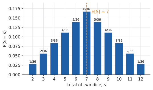
For a discrete random variable, the distribution is the list of possible values with their probabilities. Let \(S\) be the total of two dice. Counting cells in the \(6 \times 6\) grid from Chapter 29 gives:
| \(s\) | 2 | 3 | 4 | 5 | 6 | 7 | 8 | 9 | 10 | 11 | 12 |
|---|---|---|---|---|---|---|---|---|---|---|---|
\(P(S = s)\) |
\(\tfrac1{36}\) |
\(\tfrac2{36}\) |
\(\tfrac3{36}\) |
\(\tfrac4{36}\) |
\(\tfrac5{36}\) |
\(\tfrac6{36}\) |
\(\tfrac5{36}\) |
\(\tfrac4{36}\) |
\(\tfrac3{36}\) |
\(\tfrac2{36}\) |
\(\tfrac1{36}\) |
|
Probability mass function (PMF)
The probability mass function of a discrete random variable \(X\) is \(p(x) = P(X = x)\). It satisfies \(p(x) \ge 0\) for every \(x\), and \(\sum_x p(x) = 1\) (the sum over all possible values). "Mass" because each value carries a lump of probability, like beads of different weights on a number line. The support of \(X\) is the set of values with \(p(x) > 0\). |
Input: an experiment and a random variable \(X\) defined on it.
Steps:
-
List the possible values of \(X\).
-
For each value \(x\), identify the event \(X = x\) (which outcomes give that value).
-
Find its probability by counting, a tree diagram, or a known formula.
-
Check that the probabilities sum to 1.
Output: a table or formula for \(p(x) = P(X = x)\).
30.2. Expected value
30.2.1. The problem
A game costs £1 to play. You roll a die; on a 6 you win £5, otherwise nothing. Should you play? Each game is a gamble, but over a thousand games, what happens to your money?
30.2.2. Intuition: the long-run average
Over 6,000 games you’d expect about 1,000 sixes, winning \(1000 \times 5 = 5000\) pounds, while paying 6,000. You lose about £1,000, or about 17p per game. That per-game average is the expected value. It’s what the average of many repetitions settles down to (the frequency interpretation from Chapter 29, applied to quantities).
Computed directly: you win £5 with probability \(\frac16\) and £0 with probability \(\frac56\), so the average winnings per game are \(5 \times \frac16 + 0 \times \frac56 = \frac56 \approx 0.83\); subtract the £1 stake and the expected profit is \(-\frac16\) pound.
|
Expected value
The expected value (or expectation, or mean) of a discrete random variable \(X\) is
\[E[X] = \sum_x x\,P(X = x),\]
the sum of each possible value times its probability: a weighted average of the values, weighted by probability. It is often written \(\mu\) (Greek mu) or \(\mu_X\). Interpretation: the long-run average of \(X\) over many independent repetitions. |
30.2.3. Worked example: one die
Let \(X\) be the face of a fair die.
You’ll never roll 3.5. The expected value is a balance point, not a "most likely value". Picture the PMF as weights on a seesaw: \(E[X]\) is where it balances. For the two-dice total, the symmetric PMF balances at 7, so \(E[S] = 7\).
The same idea works for any function of \(X\): \(E[g(X)] = \sum_x g(x)\,P(X = x)\). For example \(E[X^2] = \frac{1 + 4 + 9 + 16 + 25 + 36}{6} = \frac{91}{6}\). Note that \(E[X^2] = 15.17 \ne (E[X])^2 = 12.25\). In general you can’t push \(E\) through a nonlinear function.
30.2.4. Linearity of expectation
The most useful fact about expectation is almost embarrassingly simple:
for any random variables \(X\) and \(Y\), whether or not they are independent.
Why it works. Think of the sample space as a finite list of outcomes \(\omega\), each with probability \(P(\omega)\). Then \(E[X] = \sum_\omega X(\omega)P(\omega)\) (group the outcomes by value and you get the earlier formula back). Now
Nothing about independence was used. A sum is a sum.
So the total of two dice has \(E[S] = E[X_1] + E[X_2] = 3.5 + 3.5 = 7\), without the PMF table. Ten dice: 35. A hundred: 350.
30.2.5. The indicator trick
Linearity becomes a superpower when combined with indicators.
|
Indicator random variable
The indicator of an event \(A\), written \(I_A\) or \(\mathbf{1}_A\), is the random variable that equals 1 if \(A\) happens and 0 otherwise. Its expectation is the probability of the event:
\[E[I_A] = 1 \cdot P(A) + 0 \cdot P(A^c) = P(A).\]
|
To find the expected number of things that happen, write the count as a sum of indicators, one per thing, and add their probabilities. You never need the distribution of the count.
Input: a random count \(X\) = "how many of the items \(1, \ldots, n\) have property \(Q\)".
Steps:
-
For each item \(i\), define \(I_i = 1\) if item \(i\) has property \(Q\), else 0. Then \(X = I_1 + I_2 + \cdots + I_n\).
-
For each \(i\), compute \(P(\text{item } i \text{ has } Q)\). Often, by symmetry, they’re all equal.
-
Add: \(E[X] = \sum_i P(\text{item } i \text{ has } Q)\).
Output: \(E[X]\). Dependence between items does not matter.
30.2.6. Worked example: the hat-check problem
\(n\) people check their hats at a restaurant. The attendant loses the tickets and hands the hats back in a uniformly random order. On average, how many people get their own hat back?
The events "person \(i\) gets their own hat" are heavily dependent (if the first \(n-1\) people all get their own hats, so does the last). Computing the distribution of the number of matches is a genuinely hard counting problem. Linearity ignores all that.
-
Let \(I_i = 1\) if person \(i\) gets their own hat. The number of matches is \(M = I_1 + \cdots + I_n\).
-
In a random permutation, person \(i\)'s hat is equally likely to go to any of the \(n\) people, so \(P(I_i = 1) = \frac1n\).
-
\(E[M] = n \times \frac1n = 1\).
Exactly one match on average, whether there are 3 people or 3 million. (A harder inclusion–exclusion argument shows that the probability of no matches tends to \(1/e \approx 0.368\).)
import random

def fixed_points(n, rng):
    hats = list(range(n))
    rng.shuffle(hats)                      # random permutation
    return sum(hats[i] == i for i in range(n))

rng = random.Random(6)
for n in (3, 10, 100):
    trials = 100_000
    results = [fixed_points(n, rng) for _ in range(trials)]
    mean = sum(results) / trials
    p_none = results.count(0) / trials
    print(f"n={n:5d}  average matches={mean:.3f}  P(no match)={p_none:.3f}")
n= 3 average matches=1.005 P(no match)=0.332 n= 10 average matches=1.005 P(no match)=0.366 n= 100 average matches=0.996 P(no match)=0.369
|
When expectation misleads
|
30.2.7. Where you’d use this
-
Everyday: is the extended warranty worth it? A £400 washing machine comes with an offer of a two-year warranty for £40. Suppose the chance of a breakdown in those two years is 5% and a typical repair costs £200. Your expected repair bill without the warranty is \(0.05 \times 200 = 10\) pounds. The warranty costs four times the repair bill it saves you on average; that gap is the seller’s profit margin. (Buying it can still be rational if a £200 surprise would genuinely hurt you, but now you know the price of that peace of mind.)
-
Chemistry: atomic masses are expectations. Chlorine is 75.8% chlorine-35 and 24.2% chlorine-37. Pick an atom at random; its expected mass is \(35 \times 0.758 + 37 \times 0.242 = 35.48\), the value printed on the periodic table. A weighted average is an expected value.
-
Computing: average memory access time. A cache hit costs 1 ns, a miss (a trip to main memory) costs 100 ns, and the hit rate is 90%. Expected access time: \(0.9 \times 1 + 0.1 \times 100 = 10.9\) ns. Raising the hit rate to 99% gives \(0.99 + 1 = 1.99\) ns, five times faster, which is why so much engineering goes into the last few percent of cache hits.
30.3. Variance and standard deviation
30.3.1. The problem
Two servers both average 100 ms per request. One always takes 95–105 ms. The other takes 10 ms most of the time and occasionally 2 seconds. The means agree; the experiences don’t. You need a number for spread.
30.3.2. Intuition and definition
Measure how far \(X\) typically lands from its mean \(\mu\). The deviation \(X - \mu\) averages to zero (positives and negatives cancel: \(E[X - \mu] = \mu - \mu = 0\)), so square it first, making every deviation count positively, then average.
|
Variance and standard deviation
The variance of \(X\), with \(\mu = E[X]\), is the expected squared deviation from the mean:
\[\operatorname{Var}(X) = E\bigl[(X - \mu)^2\bigr].\]
It is often written \(\sigma^2\) (sigma squared). The standard deviation is its square root, \(\sigma = \sqrt{\operatorname{Var}(X)}\), which has the same units as \(X\) (milliseconds rather than milliseconds squared), so it’s the one to quote. Rough meaning: \(\sigma\) is a typical distance between \(X\) and its mean. |
30.3.3. Why it works: the computing formula
Expanding the square and using linearity gives a formula that’s usually easier:
"Mean of the square minus square of the mean."
30.3.4. Worked example: one die
From before, \(E[X] = 3.5\) and \(E[X^2] = 91/6\).
A die typically lands about 1.7 away from 3.5, which matches the eye: the values 1 to 6 are between 0.5 and 2.5 from the centre.
30.3.5. Rules for variance
Adding a constant \(b\) shifts everything and doesn’t change spread; scaling by \(a\) scales deviations by \(a\), so squared deviations by \(a^2\). The sum rule needs independence (in general there’s an extra covariance term, Section 30.8). Note the consequence: for the average of \(n\) independent copies of \(X\),
Averaging \(n\) measurements shrinks the spread by a factor of \(\sqrt n\). To halve the noise, take four times as many measurements. Hold on to this: it’s the engine of the law of large numbers, the central limit theorem and nearly all of Chapter 31.
|
Variance is not additive for dependent quantities
Standard deviations never add (\(\sigma_{X + Y} \ne \sigma_X + \sigma_Y\) even for independent variables; it’s the variances that add). And if two latencies are positively correlated (same overloaded database), the variance of their sum is larger than the sum of variances. Capacity plans that assume independence underestimate bad days. |
30.3.6. Where you’d use this
-
Engineering: tolerance stacking. Three machined spacers are stacked; each has length error with standard deviation 0.1 mm, independently. The worst case adds to 0.3 mm, but the standard deviation of the total is \(\sqrt{3 \times 0.1^2} \approx 0.17\) mm, because variances add, not standard deviations. Engineers call this root-sum-square tolerancing; it lets them specify cheaper parts without over-designing for a worst case that almost never happens.
-
Lab science and sport timing: averaging four independent readings halves the standard deviation of the result (\(\sigma/\sqrt4\)). That’s why a chemistry practical asks for repeat titrations and why a hand-timed 100 m is less trustworthy than the average of several timekeepers.
-
Computing: latency budgets. A page makes three independent backend calls in sequence, each with standard deviation 20 ms. The total’s standard deviation is \(\sqrt{3} \times 20 \approx 35\) ms, not 60 ms. Variance (as "jitter") also matters in its own right: video calls and games care as much about consistent packet timing as about the average.
30.4. The named discrete distributions
A small family of distributions models a huge range of situations. Learn each as a story: if your situation matches the story, the formulas come for free.
30.4.1. Bernoulli: one yes/no trial
Story: one trial that succeeds with probability \(p\) (a coin flip, a click or not, a packet lost or not). \(X = 1\) on success, 0 on failure.
The variance: \(E[X^2] = p\) (since \(X^2 = X\) when \(X\) is 0 or 1), so \(\operatorname{Var} = p - p^2 = p(1 - p)\). It’s largest at \(p = 1/2\), the most uncertain coin.
30.4.2. Binomial: number of successes in \(n\) trials
Story: \(n\) independent Bernoulli trials, each with success probability \(p\). \(X\) = number of successes. Write \(X \sim \text{Bin}(n, p)\), read "\(X\) has the binomial distribution with parameters \(n\) and \(p\)".
Deriving the PMF by counting. Take \(n = 5\), and ask for exactly \(k = 2\) successes. One particular sequence, say SSFFF, has probability \(p \cdot p \cdot (1-p)(1-p)(1-p) = p^2(1-p)^3\) by independence. Every sequence with exactly 2 S’s and 3 F’s has the same probability, just in a different order. How many such sequences? Choose which 2 of the 5 positions are S: \(\binom52 = 10\) (Chapter 24). The sequences are disjoint, so add: \(P(X = 2) = 10\,p^2(1-p)^3\). In general:
The binomial theorem confirms these sum to \((p + (1 - p))^n = 1^n = 1\); that’s where the distribution gets its name.
Mean and variance, without algebra. \(X = X_1 + \cdots + X_n\), a sum of independent Bernoullis. By linearity \(E[X] = np\); by independence \(\operatorname{Var}(X) = np(1 - p)\).
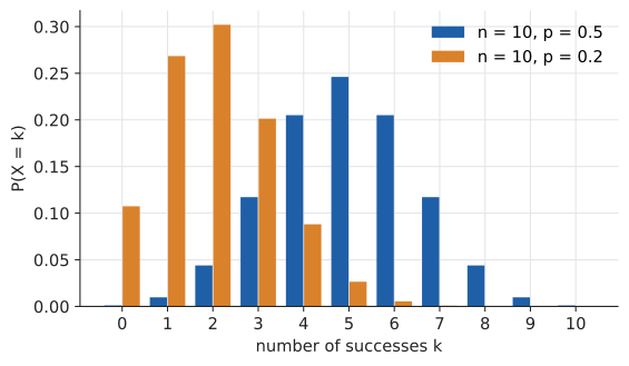
Worked example. Ten fair coin flips. Probability of exactly 7 heads? Try it: Binomial(10, 0.5) at 7.
Probability of 8 or more heads: \(\frac{\binom{10}{8} + \binom{10}{9} + \binom{10}{10}}{1024} = \frac{45 + 10 + 1}{1024} = \frac{56}{1024} \approx 0.055\).
from math import comb

def binom_pmf(k, n, p):
    return comb(n, k) * p**k * (1 - p)**(n - k)

n, p = 10, 0.5
print(round(binom_pmf(7, n, p), 4))
print(round(sum(binom_pmf(k, n, p) for k in range(8, 11)), 4))
mean = sum(k * binom_pmf(k, n, p) for k in range(n + 1))
var = sum((k - mean)**2 * binom_pmf(k, n, p) for k in range(n + 1))
print(round(mean, 6), round(var, 6))
0.1172 0.0547 5.0 2.5
The brute-force mean and variance match \(np = 5\) and \(np(1-p) = 2.5\).
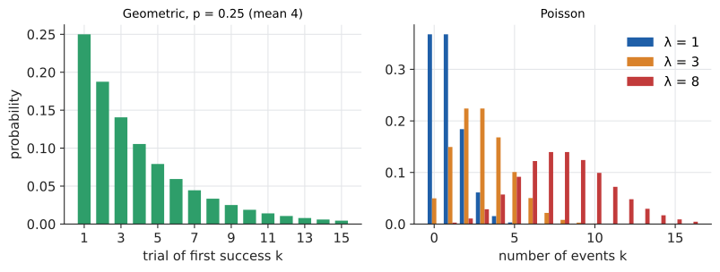
30.4.3. Geometric: waiting for the first success
Story: repeat independent trials with success probability \(p\) until the first success. \(X\) = number of trials needed (including the success).
The first success is on trial \(k\) exactly when the first \(k - 1\) trials fail and trial \(k\) succeeds:
The mean, by a conditioning trick. Let \(\mu = E[X]\). Look at the first trial. With probability \(p\) it succeeds, and you’re done after 1 trial. With probability \(1 - p\) it fails, you’ve used 1 trial, and, because trials are independent, you’re back where you started, facing another \(\mu\) trials on average. So
If a request fails with probability 0.25, so succeeds with probability \(p = 0.75\), a retry loop needs \(1/0.75 \approx 1.33\) attempts on average. Rolling a die until you get a six takes 6 rolls on average. (The variance is \((1 - p)/p^2\).)
The geometric distribution is memoryless: having already failed 10 times doesn’t make success any more likely on trial 11. That’s the gambler’s fallacy from Chapter 29 in distribution form.
30.4.4. Poisson: counting rare events
The problem. A web server receives on average 3 requests per second, from a huge population of users each of whom is very unlikely to send a request in any particular second. What’s the probability of 0 requests in a given second? Of 6 or more?
Story: count events that happen independently, at a constant average rate, where each tiny time slice has only a tiny chance of an event. \(X \sim \text{Poisson}(\lambda)\), where \(\lambda\) (lambda) is the average count per interval:
Where it comes from. Chop the second into \(n\) tiny slices, each containing a request with probability \(p = \lambda/n\). The count is binomial, \(\text{Bin}(n, \lambda/n)\). As \(n \to \infty\) with \(np = \lambda\) fixed,
by the compound-interest limit from Chapter 12, and similar limits give the other terms. So the Poisson is the binomial for "many trials, each rare". Numerically: \((1 - 3/1000)^{1000} \approx 0.0496\), already close to \(e^{-3} \approx 0.0498\).
Worked example. With \(\lambda = 3\): Try it: Poisson with λ = 3.
About 1 second in 20 sees no traffic, and about 1 in 12 sees double the average or more. If the server can handle 5 requests per second, it will be overloaded 8% of the time, even though the average load is only 60% of capacity. Randomness creates queues.
30.4.5. Choosing a discrete model
| Question | Distribution | Typical use |
|---|---|---|
Did one trial succeed? |
Bernoulli(\(p\)) |
a click, a bit flip, a test pass |
How many successes in \(n\) fixed, independent trials? |
Binomial(\(n, p\)) |
conversions out of \(n\) visitors; defective chips in a batch |
How many trials until the first success? |
Geometric(\(p\)) |
retries until success; attempts until a hash finds an empty slot |
How many events in a fixed interval, at a constant rate? |
Poisson(\(\lambda\)) |
requests per second, typos per page, mutations per genome |
Every one of \(n\) values equally likely? |
Discrete uniform |
dice, random array index, shuffles |
|
Model assumptions
Every named distribution packages assumptions. Binomial needs a fixed number of trials with the same \(p\) and independence; users who visit twice, or a \(p\) that varies by user, break it. Poisson needs a constant rate and independent events; real traffic has daily cycles and bursts (one tweet sends thousands of users at once), so the variance of real request counts is often far larger than the mean. A quick diagnostic: for count data, if the sample variance is much bigger than the sample mean, a Poisson model is wrong. |
|
Why "Poisson"? And the Prussian cavalry
Siméon Denis Poisson derived the distribution in 1837 while studying wrongful convictions. Its most famous early application was by Ladislaus Bortkiewicz in 1898, who showed that the number of Prussian cavalrymen killed by horse kicks per corps per year (20 years, 14 corps) fitted a Poisson distribution with \(\lambda \approx 0.7\) almost perfectly. The same mathematics now counts photon arrivals in a camera sensor, radioactive decays, and packets arriving at a router. |
30.4.6. Where you’d use this
-
Sport (Poisson). Football goals are rare, roughly independent events: a typical top-flight match averages about 2.7 goals. Treating the total as Poisson(2.7), \(P(\text{0--0}) = e^{-2.7} \approx 0.067\) and \(P(\text{at most 1 goal}) = e^{-2.7}(1 + 2.7) \approx 0.25\). Betting companies price their odds from models built on exactly this, with a separate rate for each team.
-
Manufacturing and medicine (binomial). A production line makes chips with a 2% defect rate. In a batch of 20, \(P(\text{no defects}) = 0.98^{20} \approx 0.67\), so a third of batches contain at least one dud: that’s how acceptance-sampling plans are set. Clinical trials use the same model: "how many of 200 patients will respond if the true rate is 30%?" is a \(\text{Bin}(200, 0.3)\) question, with mean 60 and standard deviation \(\sqrt{42} \approx 6.5\).
-
Computing (binomial): replication. A database keeps 3 replicas, each independently down 1% of the time. All three are down with probability \(0.01^3 = 10^{-6}\). A majority-quorum write needs at least 2 of 3 up: it fails if 2 or more are down, with probability \(3(0.01)^2(0.99) + 0.01^3 \approx 0.0003\), so availability is 99.97%. (The independence assumption is the weak point: replicas in the same data centre fail together.)
-
Computing (geometric): retries. A flaky network call succeeds 75% of the time. The number of attempts is geometric, so expect \(1/0.75 \approx 1.33\) attempts, and the chance of needing more than 3 is \(0.25^3 \approx 1.6\%\). That’s how you choose a retry limit.
30.5. Continuous distributions
30.5.1. The problem
How long until the next request arrives? It could be 0.3 s, 0.31 s, 0.3141 s: any real number. Now ask "what’s the probability it’s exactly 0.3 seconds, to infinitely many decimal places?". There are infinitely many possible values; if each had positive probability, the total would be infinite. So each individual value must have probability 0. Yet "between 0.2 and 0.4 seconds" clearly has positive probability. Lists of probabilities can’t work; we need a different description.
30.5.2. Intuition: probability as area
Think of a histogram of a million measured waiting times, with very narrow bins, scaled so the total area of the bars is 1. The probability of landing in any range is the area of the bars over that range. As the bins get narrower, the bar tops trace out a smooth curve: the probability density function. Probability is area under it.
|
Probability density function (PDF)
A continuous random variable \(X\) has a probability density function \(f(x)\) if
\[P(a \le X \le b) = \text{area under } f \text{ between } a \text{ and } b \quad \left(= \int_a^b f(x)\,dx\right).\]
(The integral notation is from Chapter 19; "area under the curve" is all you need here.) A density satisfies \(f(x) \ge 0\) and has total area 1. The height \(f(x)\) is not a probability (it can exceed 1); it’s probability per unit length, like population density is people per square mile. For a short interval of width \(\Delta x\), \(P(x \le X \le x + \Delta x) \approx f(x)\,\Delta x\). For a continuous variable, \(P(X = a) = 0\) for every single value \(a\), so \(P(a \le X \le b) = P(a < X < b)\): endpoints don’t matter. |
30.5.3. Cumulative distribution functions
One description works for discrete and continuous variables alike.
|
Cumulative distribution function (CDF)
The cumulative distribution function of \(X\) is
\[F(x) = P(X \le x).\]
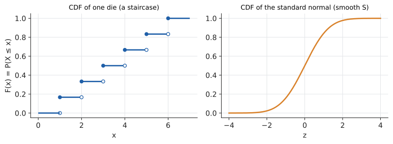
It rises from 0 (far left) to 1 (far right) and never decreases. Then \(P(a < X \le b) = F(b) - F(a)\). For a discrete variable \(F\) is a staircase, jumping by \(p(x)\) at each value; for a continuous one it’s a smooth curve whose slope is the density (\(f = F'\), Chapter 17). The median is the value where \(F(x) = 0.5\); more generally the \(q\)-th quantile (or \(100q\)-th percentile) is where \(F(x) = q\). "p99 latency" is the 0.99 quantile. |
30.5.4. Uniform: equally likely anywhere in an interval
Story: \(X\) is equally likely to land anywhere in \(\lbrack a, b]\). The density is flat: \(f(x) = \frac{1}{b - a}\) on the interval (so the rectangle has area 1), and 0 outside. Probabilities are proportional to length: \(P(c \le X \le d) = \frac{d - c}{b - a}\). The mean is the midpoint \(\frac{a + b}{2}\), and the variance is \(\frac{(b - a)^2}{12}\).
The standard uniform, on \(\lbrack 0, 1]\), is what random.random() approximates, and as you’ll see in [sec-dist-sampling], every other distribution can be built from it.
30.5.5. Exponential: waiting times
Story: the waiting time until the next event in a Poisson process with rate \(\lambda\) events per unit time. The time until the next request, the next radioactive decay, the next failure of a component that doesn’t age.
Deriving it from Poisson. The wait \(T\) exceeds \(t\) exactly when there are zero events in \(\lbrack 0, t]\). In time \(t\) the count is Poisson with mean \(\lambda t\), so
The density is the slope of \(F\): \(f(t) = \lambda e^{-\lambda t}\) for \(t \ge 0\). The mean is \(1/\lambda\) (at 3 requests per second, the average gap is a third of a second), and the standard deviation is also \(1/\lambda\).
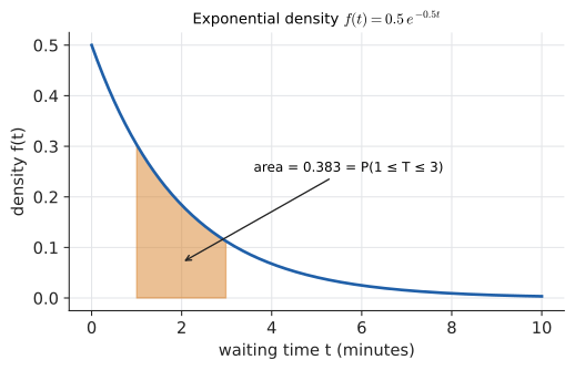
Worked example. Buses arrive as a Poisson process at rate \(\lambda = 0.5\) per minute. What’s the probability your wait is between 1 and 3 minutes? Try it: Exponential waiting time.
Memorylessness. \(P(T > s + t \mid T > s) = \frac{e^{-\lambda(s + t)}}{e^{-\lambda s}} = e^{-\lambda t} = P(T > t)\). If you’ve already waited 10 minutes, the remaining wait has the same distribution as if you’d just arrived. That’s right for radioactive atoms and for well-behaved request streams, and wrong for things that wear out (hard disks, people), which need other models.
|
Optional: expectation as an integral
(Uses Chapter 19; skip freely.) For a continuous variable the sum \(\sum x\,p(x)\) becomes an integral:
\[E[X] = \int_{-\infty}^{\infty} x f(x)\,dx, \qquad \operatorname{Var}(X) = \int_{-\infty}^{\infty} (x - \mu)^2 f(x)\,dx.\]
For the exponential, integrating by parts: \(\int_0^\infty t\,\lambda e^{-\lambda t}\,dt = \left[-t e^{-\lambda t}\right]_0^\infty + \int_0^\infty e^{-\lambda t}\,dt = 0 + \frac1\lambda\). Every rule from the discrete case (linearity, the variance formulas) carries over unchanged. |
30.5.6. Where you’d use this
-
Physics: radioactive decay and half-life. Each atom’s lifetime is exponential with rate \(\lambda\). The half-life is the median lifetime, where \(e^{-\lambda t} = \tfrac12\), i.e. \(t_{1/2} = \ln 2 / \lambda\). For carbon-14, \(t_{1/2} = 5730\) years, so \(\lambda = \ln 2 / 5730 \approx 1.21 \times 10^{-4}\) per year, the number behind radiocarbon dating.
-
Reliability engineering. A component with a constant failure rate and a mean time between failures (MTBF) of 50,000 hours survives a year of continuous use (8,760 hours) with probability \(e^{-8760/50000} \approx 0.84\). A rack of 100 such components can expect about 16 of them to fail within the year, which is how spare-parts stock and on-call rotas are planned.
-
Computing: simulation and load testing. To mimic real users arriving at 3 per second, a load generator sleeps for exponentially distributed gaps with mean 1/3 s (generated as in [sec-dist-sampling]), not for exactly 1/3 s. Evenly spaced test traffic never produces the bursts that make real queues form.
-
Uniform: rounding a measurement to the nearest millimetre leaves an error that is uniform on \(\lbrack -0.5, 0.5]\) mm, with standard deviation \(1/\sqrt{12} \approx 0.29\) mm; the same formula gives the "quantization noise" of an analogue-to-digital converter.
30.6. The normal distribution
30.6.1. The problem
Measure the heights of 10,000 adults, the errors of 10,000 repeated measurements of a length, or the average response time across 10,000 batches of requests. Plot histograms, and the same symmetric bell shape keeps appearing. Why one shape, and how do you compute with it?
The "why" is the central limit theorem (Section 30.7): any quantity that is the sum of many small, independent contributions comes out approximately bell-shaped. First, the "how".
30.6.2. The bell curve
|
Normal distribution
The normal (or Gaussian) distribution with mean \(\mu\) and standard deviation \(\sigma\), written \(N(\mu, \sigma^2)\), has density
\[f(x) = \frac{1}{\sigma\sqrt{2\pi}}\, e^{-\frac{(x - \mu)^2}{2\sigma^2}}.\]
It is symmetric about \(\mu\) (mean = median = mode), bell-shaped, and its tails thin out very fast. The standard normal is \(Z \sim N(0, 1)\); its CDF is written \(\Phi(z)\) (capital phi). The \(\sqrt{2\pi}\) makes the total area 1. Note: the second parameter in \(N(\mu, \sigma^2)\) is the variance. \(N(100, 225)\) has standard deviation 15. |
You don’t need to work with the formula directly. Two facts do almost all the work.
Standardizing. If \(X \sim N(\mu, \sigma^2)\), then
\(Z\) (the z-score) counts how many standard deviations \(X\) is from its mean. So every normal question becomes a question about one curve.
The 68–95–99.7 rule. For any normal distribution, about 68% of the probability lies within \(1\sigma\) of the mean, 95% within \(2\sigma\), and 99.7% within \(3\sigma\).
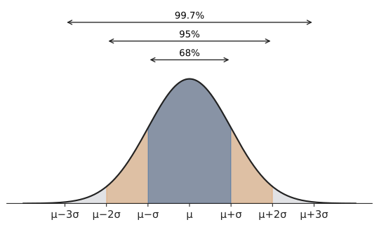
Input: \(X \sim N(\mu, \sigma^2)\) and an interval.
Steps:
-
Convert each endpoint \(x\) to a z-score: \(z = (x - \mu)/\sigma\).
-
Sketch the bell curve and shade the region you want. Decide whether it’s a left tail, right tail, or middle.
-
Use \(\Phi\) (a table, a calculator, or code): left tail \(\Phi(z)\); right tail \(1 - \Phi(z)\); middle \(\Phi(z_2) - \Phi(z_1)\). For a quick estimate, use 68–95–99.7.
-
Check the answer against the sketch (a right tail beyond \(z = 2\) must be small).
Output: the probability.
Worked example. IQ scores are scaled to be approximately \(N(100, 15^2)\). What fraction score above 130? Try it: Normal tail above 130.
Quick check with the rule: 95% lie within \(\pm 2\sigma\), so 5% lie outside, half of it above: 2.5%. ✓
from math import erf, sqrt

def normal_cdf(x, mu=0.0, sigma=1.0):
    """P(X <= x) for X ~ N(mu, sigma^2)."""
    z = (x - mu) / sigma
    return 0.5 * (1 + erf(z / sqrt(2)))

for k in (1, 2, 3):
    print(k, round(normal_cdf(k) - normal_cdf(-k), 4))
print(round(1 - normal_cdf(130, 100, 15), 4))
print(round(normal_cdf(250, 200, 40) - normal_cdf(150, 200, 40), 4))
1 0.6827 2 0.9545 3 0.9973 0.0228 0.7887
(The function erf, the error function, is in Python’s math module; \(\Phi(z) = \tfrac12\bigl(1 + \operatorname{erf}(z/\sqrt2)\bigr)\). The last line computes \(P(150 \le X \le 250)\) for \(X \sim N(200, 40^2)\), i.e. \(P(-1.25 \le Z \le 1.25)\).)
|
Not everything is normal
Request latencies, file sizes, incomes and city populations are strongly right-skewed with long tails. Modelling them as normal predicts negative latencies and badly underestimates extreme values: under a normal model, a value 6 standard deviations above the mean has probability about one in a billion; in real latency data such outliers happen daily. Always plot the data before assuming a bell curve. Monitoring uses percentiles (p50, p99, p99.9) precisely because they don’t assume a shape. |
|
Gauss and the ten-mark note
The normal curve was first found by Abraham de Moivre in 1733 as an approximation to the binomial distribution for large \(n\). Carl Friedrich Gauss used it around 1809 to model errors in astronomical observations, which is why it’s often called Gaussian. Germany’s old 10-Deutsche-Mark banknote carried Gauss’s portrait with the bell curve and its formula printed beside him. |
30.6.3. Where you’d use this
-
Shopping and the law: filling packets. A machine fills crisp packets labelled 25 g with weights that are approximately \(N(26, 0.5^2)\). The fraction under the label weight is \(P(X < 25) = P(Z < -2) \approx 2.3\%\). Setting the machine’s target is a z-score calculation: aim too low and you break trading-standards rules, too high and you give product away.
-
Medicine: reference ranges. A blood-test "normal range" is usually the middle 95% of healthy people, mean \(\pm 2\) standard deviations. The flip side: a perfectly healthy person who has 20 independent tests can expect \(20 \times 0.05 = 1\) result flagged as "abnormal".
-
Computing: sensor noise is modelled as Gaussian in GPS filters and robotics; image "Gaussian blur" weights neighbouring pixels by a bell curve; neural-network weights are initialised with small normal random numbers; and anomaly detectors raise an alert when a metric’s z-score passes 3, while remembering the watch-out above about heavy tails.
30.7. The law of large numbers and the central limit theorem
30.7.1. The problem
A single die roll is unpredictable. The average of 10,000 rolls is extremely predictable: it will be very close to 3.5. A single user’s session length is unpredictable; the mean session length across a million users barely moves day to day. Why does averaging tame randomness, and how fast?
30.7.2. The law of large numbers
Let \(X_1, X_2, \ldots, X_n\) be independent random variables, all with the same distribution (independent and identically distributed, or i.i.d.), with mean \(\mu\) and standard deviation \(\sigma\). Their sample mean is
(\(\bar X\) is read "X-bar".) We computed in Section 30.3 that \(E[\bar X_n] = \mu\) and \(\operatorname{SD}(\bar X_n) = \sigma/\sqrt n\). As \(n\) grows, the spread of the average around \(\mu\) shrinks to zero. That is the law of large numbers: the sample mean converges to the true mean.
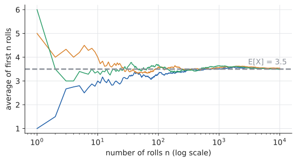
To make "converges" precise, Chebyshev’s inequality says that any random variable is unlikely to be many standard deviations from its mean: \(P(|Y - E[Y]| \ge k\sigma_Y) \le 1/k^2\). Applied to \(\bar X_n\), with a fixed tolerance \(\varepsilon\) (epsilon, a small positive number), Try it: Run the law of large numbers.
This is why the frequentist interpretation of probability (Chapter 29) is coherent: the proportion of heads is the sample mean of Bernoulli indicators, so it converges to \(p\). Try it: Proportion of heads converging.
30.7.3. The central limit theorem
The law of large numbers says the sample mean concentrates around \(\mu\). The central limit theorem (CLT) says what shape its fluctuations have: approximately normal, no matter what distribution the individual \(X_i\) have (provided their variance is finite).
|
Central limit theorem
If \(X_1, \ldots, X_n\) are i.i.d. with mean \(\mu\) and standard deviation \(\sigma\), then for large \(n\),
\[\bar X_n \ \approx\ N\!\left(\mu,\ \frac{\sigma^2}{n}\right), \qquad\text{equivalently}\qquad \frac{\bar X_n - \mu}{\sigma/\sqrt n} \approx N(0, 1).\]
The sum \(X_1 + \cdots + X_n\) is likewise approximately \(N(n\mu, n\sigma^2)\). The quantity \(\sigma/\sqrt n\) is the standard error of the mean. |
Watch it happen with an extremely un-normal starting distribution, the exponential (all mass on the positive side, a long right tail):
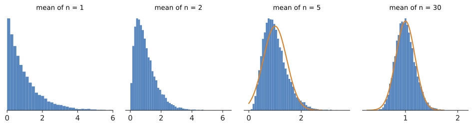
Why should sums become normal? A rough intuition: each extra term adds a small independent nudge; the fine details of each nudge’s distribution wash out, and only the mean and variance survive. A sum of many small independent nudges is the situation the normal distribution describes. (The full proof uses more machinery than this book develops.) Try it: Build the bell curve yourself; Exponential means, n = 1.
import numpy as np

rng = np.random.default_rng(12)
print("  n   sd of means   1/sqrt(n)   below -1.96 SE   above +1.96 SE")
for n in (1, 5, 30, 100):
    # 100,000 experiments, each the mean of n exponential(1) values
    means = rng.exponential(1.0, size=(100_000, n)).mean(axis=1)
    se = 1 / np.sqrt(n)              # population sd is 1
    below = np.mean(means < 1 - 1.96 * se)
    above = np.mean(means > 1 + 1.96 * se)
    print(f"{n:3d}   {means.std():.3f}         {se:.3f}       "
          f"{below:.3f}            {above:.3f}")
n sd of means 1/sqrt(n) below -1.96 SE above +1.96 SE 1 1.001 1.000 0.000 0.052 5 0.448 0.447 0.000 0.044 30 0.182 0.183 0.014 0.033 100 0.100 0.100 0.019 0.029
Read the output carefully. The standard deviation of the mean matches \(\sigma/\sqrt n\) exactly at every \(n\): that part is not an approximation. The shape approaches normal more slowly. For a normal distribution, 2.5% would fall in each tail beyond \(\pm 1.96\) standard errors; with skewed data, even at \(n = 30\) the tails are lopsided (1.4% versus 3.3%).
|
The limits of the limit theorems
|
|
Galton’s bean machine
Francis Galton built a device in the 1870s, the quincunx: beads fall through rows of pins, bouncing left or right at each one, and pile up in bins at the bottom. Each bead’s final position is a sum of many independent ±1 bounces, a binomial variable, and the pile forms a bell curve every time. Galton wrote that the law "would have been personified by the Greeks and deified, if they had known of it". |
30.7.4. Where you’d use this
-
Casinos and insurers. A bet of £1 on red in European roulette wins £1 with probability \(\tfrac{18}{37}\) and loses £1 with probability \(\tfrac{19}{37}\): mean \(-\tfrac1{37}\) pound, standard deviation almost exactly £1. Over a million such bets the casino’s expected profit is \(10^6/37 \approx 27{,}000\) pounds and, by the CLT, its standard deviation is only about \(\sqrt{10^6} \times 1 = 1{,}000\) pounds. A loss would be a 27-standard-deviation event. Gamblers face randomness; the house faces arithmetic. Insurance works the same way.
-
Opinion polls. Ask 1,000 random voters. If support is near 50%, each answer is a Bernoulli with standard deviation 0.5, so the poll’s standard error is \(0.5/\sqrt{1000} \approx 0.016\), and \(\pm 1.96\) standard errors is the familiar "margin of error ±3%". To get ±1% you need about 9,600 people: the \(\sqrt n\) law again (Chapter 31).
-
Computing: Monte Carlo and A/B tests. A Monte Carlo estimate (rendering a pixel by averaging random light paths, pricing an option, estimating \(\pi\)) has error proportional to \(1/\sqrt n\): 100 times more samples for one more correct digit. The same law tells an A/B test how many users it needs before a 1% difference in click rate stands out from the noise.
|
Build your own bell curve
Choose any starting distribution, including a die, an exponential, a two-spike "0 or 100" distribution, or one you draw by hand. Choose \(n\). The lab draws thousands of samples of size \(n\) and builds the histogram of their means live, overlaying the predicted normal curve \(N(\mu, \sigma^2/n)\). A tail meter shows the fraction outside \(\pm 1.96\) standard errors versus the normal’s 5%. Then switch to a Cauchy distribution and watch the CLT fail. |
30.8. Joint distributions, covariance and correlation
30.8.1. The problem
Do slower pages have higher bounce rates? Does CPU load rise with request count? These questions are about two random variables at once and whether they move together.
30.8.2. Joint distributions
The joint distribution of discrete \(X\) and \(Y\) gives \(P(X = x, Y = y)\) (the comma means "and") for every pair of values. It’s a two-way table, exactly like the deploy table in Chapter 29.
Example. Roll a die. Let \(X = 1\) if the roll is even (else 0), and \(Y = 1\) if the roll is at least 4 (else 0). Rolls: 1 → (0,0), 2 → (1,0), 3 → (0,0), 4 → (1,1), 5 → (0,1), 6 → (1,1).
| \(Y = 0\) | \(Y = 1\) | \(P(X = x)\) | |
|---|---|---|---|
\(X = 0\) |
\(2/6\) |
\(1/6\) |
\(1/2\) |
\(X = 1\) |
\(1/6\) |
\(2/6\) |
\(1/2\) |
\(P(Y = y)\) |
\(1/2\) |
\(1/2\) |
1 |
The row and column totals, written in the margins, are the marginal distributions of \(X\) and \(Y\) on their own. \(X\) and \(Y\) are independent if every cell equals the product of its marginals: \(P(X = x, Y = y) = P(X = x)P(Y = y)\). Here \(P(X = 1, Y = 1) = 2/6 \ne \frac12 \cdot \frac12\), so they’re dependent: knowing the roll is even makes "at least 4" more likely.
30.8.3. Covariance
|
Covariance
The covariance of \(X\) and \(Y\), with means \(\mu_X\) and \(\mu_Y\), is
\[\operatorname{Cov}(X, Y) = E\bigl[(X - \mu_X)(Y - \mu_Y)\bigr] = E[XY] - \mu_X \mu_Y.\]
Positive when \(X\) and \(Y\) tend to be above (or below) their means together; negative when one tends to be high as the other is low; zero (uncorrelated) when there’s no linear tendency. \(\operatorname{Cov}(X, X) = \operatorname{Var}(X)\). Variance of a sum, in general: \(\operatorname{Var}(X + Y) = \operatorname{Var}(X) + \operatorname{Var}(Y) + 2\operatorname{Cov}(X, Y)\). |
Why the product? If both deviations have the same sign, their product is positive; if opposite signs, negative. Averaging the products measures which tendency wins.
For the die example: \(E[XY] = P(X = 1, Y = 1) = \frac26 = \frac13\) (since \(XY\) is 1 only when both are 1), and \(\mu_X = \mu_Y = \frac12\). So \(\operatorname{Cov}(X, Y) = \frac13 - \frac14 = \frac1{12}\): positive, as expected.
30.8.4. Correlation
Covariance has awkward units (milliseconds times bounces) and depends on scale. Dividing by both standard deviations gives a pure number between \(-1\) and 1:
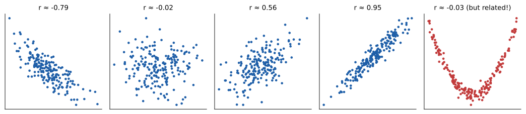
\(\rho\) (rho) is the correlation coefficient. \(\rho = 1\) means \(Y\) is an exact increasing linear function of \(X\); \(\rho = -1\), an exact decreasing one; \(\rho = 0\), no linear relationship. For the die example, \(\sigma_X = \sigma_Y = \sqrt{\frac12 \cdot \frac12} = \frac12\), so \(\rho = \frac{1/12}{1/4} = \frac13\).
|
Uncorrelated does not mean independent
Independent variables always have zero covariance (\(E[XY] = E[X]E[Y]\) under independence). The converse fails: in the last scatter plot \(Y\) is almost determined by \(X\), yet \(\rho \approx 0\), because the upward and downward halves cancel. Correlation measures linear association only. And correlation is not causation; that’s a theme of Chapter 31. |
30.8.5. Where you’d use this
-
Finance: why diversification works. Put half your money in each of two investments, each with yearly return standard deviation 10%. Using \(\operatorname{Var}(\tfrac12 X + \tfrac12 Y) = \tfrac14\sigma_X^2 + \tfrac14\sigma_Y^2 + \tfrac12\rho\,\sigma_X\sigma_Y\), the portfolio’s standard deviation is 10% if \(\rho = 1\), about 7.1% if \(\rho = 0\), and 5% if \(\rho = -0.5\). Diversification buys you risk reduction only to the extent that the investments are not correlated, which is why crashes, when everything falls together, hurt so much.
-
Science: finding relationships. Epidemiologists start with correlations (smoking and lung cancer, height of parents and children) and then work hard to rule out confounders before claiming cause (Chapter 31).
-
Computing: recommender systems measure how strongly two users' ratings are correlated ("people like you also liked…"); monitoring dashboards flag metrics that suddenly become correlated (latency and one particular host); and the covariance matrix in the sidebar below drives PCA.
30.9. Distributions at work in computing
30.9.1. Expected running time
Linear search. Search an array of \(n\) distinct items for one that’s equally likely to be in any position. The number of comparisons is uniform on \(\{1, \ldots, n\}\), so the expected number is \(\frac{1 + 2 + \cdots + n}{n} = \frac{n + 1}{2}\).
Hash table chains. Insert \(n\) keys into \(m\) buckets with a good hash. For a given bucket, the number of keys in it is a sum of \(n\) indicators each with probability \(1/m\), so by linearity its expected length is \(n/m\), the load factor \(\alpha\). An unsuccessful lookup scans a chain of expected length \(\alpha\): constant time if you keep \(\alpha\) bounded by resizing.
Randomized quicksort (promised in Chapter 29). Let the sorted values be \(z_1 < z_2 < \cdots < z_n\). Quicksort only ever compares an element with the current pivot, and any pair is compared at most once. Let \(I_{ij} = 1\) if \(z_i\) and \(z_j\) (\(i < j\)) are ever compared. Total comparisons \(C = \sum_{i<j} I_{ij}\).
Focus on the block \(z_i, z_{i + 1}, \ldots, z_j\) (\(j - i + 1\) values). Until a pivot is chosen from this block, all of them stay together in the same subarray. When the first pivot from the block is chosen, if it’s \(z_i\) or \(z_j\), those two get compared; if it’s anything in between, they’re split into different subarrays and never meet. Every element of the block is equally likely to be that first pivot, so
where \(H_n = 1 + \frac12 + \frac13 + \cdots + \frac1n \approx \ln n + 0.577\) is the \(n\)-th harmonic number. (The exact value is \(2(n + 1)H_n - 4n\).) No input is bad; only the coin flips are random.
import random

def quicksort_comparisons(a, rng):
    """Return number of comparisons randomized quicksort makes on list a."""
    if len(a) <= 1:
        return 0
    pivot = a[rng.randrange(len(a))]
    less = [x for x in a if x < pivot]
    more = [x for x in a if x > pivot]
    # every non-pivot element is compared with the pivot once
    return (len(a) - 1) + quicksort_comparisons(less, rng) \
                        + quicksort_comparisons(more, rng)

n = 1000
H = sum(1 / k for k in range(1, n + 1))
exact = 2 * (n + 1) * H - 4 * n
rng = random.Random(7)
runs = [quicksort_comparisons(list(range(n)), rng) for _ in range(200)]
print(round(exact, 1), sum(runs) / len(runs))
10985.9 10957.005
The input list(range(n)) is already sorted, the worst case for a first-element pivot (about 500,000 comparisons); with random pivots it costs about 11,000.
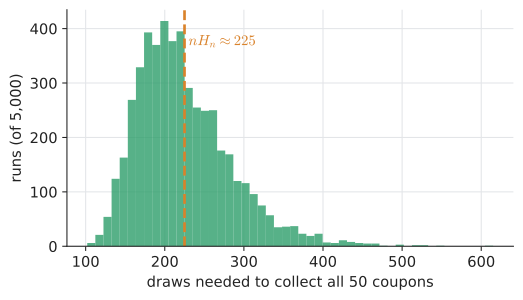
Try it: Collect 50 coupons. ==== The coupon collector
The problem. A cereal brand puts one of \(n\) equally likely toys in each box. How many boxes until you have all \(n\)? The same question: how many random requests until every one of \(n\) servers has been hit; how many random tests until every one of \(n\) code paths is covered.
The method. Split the process into phases. Phase \(k\) starts when you have \(k - 1\) distinct toys and ends when you get a new one. During phase \(k\), each box is new with probability \(p_k = \frac{n - k + 1}{n}\), so the phase length is geometric with mean \(\frac{n}{n - k + 1}\). By linearity,
For \(n = 50\): \(50 \times H_{50} \approx 50 \times 4.499 = 225\) boxes. The last toy alone takes 50 boxes on average; the first takes 1.
import random

def draws_to_collect(n, rng):
    seen, draws = set(), 0
    while len(seen) < n:
        seen.add(rng.randrange(n))
        draws += 1
    return draws

n = 50
H = sum(1 / k for k in range(1, n + 1))
rng = random.Random(8)
sim = sum(draws_to_collect(n, rng) for _ in range(20_000)) / 20_000
print(round(n * H, 2), round(sim, 2))
224.96 224.48
Try it: Balls into bins, two choices. ==== Balls into bins: load balancing
Throw \(n\) requests (balls) at \(n\) servers (bins) uniformly at random.
-
Expected load per server: exactly 1, by linearity.
-
Expected fraction of idle servers: a given server misses every ball with probability \((1 - \frac1n)^n \approx e^{-1} \approx 0.368\). So about 37% of servers sit idle while others are double- or triple-loaded.
-
Maximum load: grows slowly, like \(\frac{\ln n}{\ln \ln n}\), but it does grow.
The power of two choices: for each ball, pick two random bins and put the ball in the less loaded one. This tiny change cuts the maximum load to about \(\frac{\ln \ln n}{\ln 2}\), an exponential improvement. It’s used in real load balancers (for example, NGINX’s random two method) and in hash tables (cuckoo hashing).
import random

def max_load(n, choices, rng):
    bins = [0] * n
    for _ in range(n):
        if choices == 1:
            b = rng.randrange(n)
        else:
            c1, c2 = rng.randrange(n), rng.randrange(n)
            b = c1 if bins[c1] <= bins[c2] else c2
        bins[b] += 1
    return max(bins), bins.count(0) / n

rng = random.Random(9)
n = 100_000
print("one choice :", max_load(n, 1, rng))
print("two choices:", max_load(n, 2, rng))
one choice : (8, 0.36719) two choices: (4, 0.23785)
Try it: Inverse-transform sampling, animated. ==== Sampling from a distribution: inverse transform sampling
The problem. Your language gives you random(), uniform on \(\lbrack 0, 1)\). A simulation needs exponential inter-arrival times, or a weighted choice among options. How do you turn uniform randomness into any distribution?
Intuition. Look at the CDF \(F\). It maps values to probabilities in \(\lbrack 0, 1]\). Run it backwards: pick a height \(u\) uniformly on the vertical axis, move across to the curve, and drop down to the \(x\) axis. Where the CDF is steep (high density), a wide band of heights maps to a narrow band of \(x\), so those \(x\) values get picked often. Exactly right.
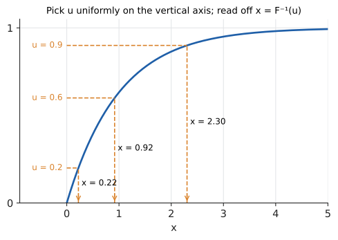
Why it works. Let \(U\) be uniform on \(\lbrack 0,1]\) and \(X = F^{-1}(U)\) (the inverse function, Chapter 11). Since \(F\) is increasing, \(X \le x\) exactly when \(U \le F(x)\), so \(P(X \le x) = P(U \le F(x)) = F(x)\): the uniform’s CDF is \(P(U \le u) = u\). So \(X\) has CDF \(F\), as required.
For the exponential, solve \(u = 1 - e^{-\lambda x}\) for \(x\):
For a discrete distribution, the CDF is a staircase, and "inverting" it means: walk up the staircase until the cumulative probability first exceeds \(u\). Try it: Walk up the CDF staircase.
Input: a target distribution with CDF \(F\); a source of uniform random numbers on \(\lbrack 0, 1)\).
Steps:
-
Draw \(u\) uniformly from \(\lbrack 0, 1)\).
-
Continuous case: solve \(F(x) = u\) for \(x\) (by algebra if possible, else numerically, as in Chapter 32) and return \(x = F^{-1}(u)\).
-
Discrete case: with values \(v_1, v_2, \ldots\) and probabilities \(p_1, p_2, \ldots\), accumulate \(c = p_1 + p_2 + \cdots\) and return the first \(v_i\) for which \(u < c\).
-
Repeat for each sample needed (fresh \(u\) each time).
Output: samples with distribution \(F\).
import math, random

def sample_exponential(rate, rng=random):
    u = rng.random()                 # uniform on [0, 1)
    return -math.log(1 - u) / rate   # inverse of F(x) = 1 - exp(-rate x)

def sample_discrete(values, probs, rng=random):
    u = rng.random()
    cumulative = 0.0
    for v, p in zip(values, probs):
        cumulative += p              # walk up the CDF staircase
        if u < cumulative:
            return v
    return values[-1]                # guard against rounding

random.seed(10)
xs = [sample_exponential(0.5) for _ in range(100_000)]
print(round(sum(xs) / len(xs), 3))                     # should be near 1/0.5 = 2
print(round(sum(x > 3 for x in xs) / len(xs), 3), round(math.exp(-1.5), 3))
draws = [sample_discrete(["a", "b", "c"], [0.5, 0.3, 0.2]) for _ in range(100_000)]
print({v: round(draws.count(v) / len(draws), 3) for v in "abc"})
1.994
0.223 0.223
{'a': 0.499, 'b': 0.302, 'c': 0.199}
Alternatives and choosing. Inverse transform is the default whenever \(F^{-1}\) has a formula. The normal distribution doesn’t, so libraries use special methods (the Box–Muller transform, or the faster ziggurat algorithm). For discrete distributions with many values sampled many times, the linear walk is slow; use binary search on the cumulative array (\(O(\log n)\), this is what Python’s random.choices does) or the alias method (\(O(1)\) per sample after setup). Rejection sampling handles densities you can evaluate but not invert.
|
Using 1 − u, not u
|
Try it: Step through reservoir sampling. ==== Reservoir sampling
The problem. Choose \(k\) items uniformly at random from a stream (log lines, tweets, packets) whose length you don’t know in advance and which is too big to store. You get one pass.
The method (Algorithm R). Keep the first \(k\) items in a "reservoir". For the \(i\)-th item (\(i > k\)), keep it with probability \(k/i\), replacing a uniformly random reservoir slot.
Why it works (the case \(k = 1\)). Keep item \(i\) with probability \(1/i\). Item \(i\) survives to the end of a stream of length \(n\) if it’s chosen at step \(i\) and not replaced at any later step \(i + 1, \ldots, n\):
Every item ends up equally likely, whatever \(n\) turns out to be. The general-\(k\) argument is the same with \(k/i\) and a factor \((1 - \frac{1}{j})\) for "replaced at step \(j\) and that slot was mine", and gives \(k/n\) for every item (an induction proof, Chapter 22).
import random
from collections import Counter

def reservoir_sample(stream, k, rng=random):
    """Uniform random sample of k items from an iterable of unknown length."""
    reservoir = []
    for i, item in enumerate(stream, start=1):   # i = items seen so far
        if i <= k:
            reservoir.append(item)
        else:
            j = rng.randrange(i)                 # 0 .. i-1
            if j < k:                            # happens with prob k/i
                reservoir[j] = item
    return reservoir

random.seed(11)
counts = Counter()
for _ in range(100_000):
    counts.update(reservoir_sample(range(10), 3))
print([round(counts[x] / 100_000, 3) for x in range(10)])   # each ~ 0.3
[0.301, 0.299, 0.3, 0.301, 0.301, 0.3, 0.299, 0.298, 0.3, 0.299]
Each of the 10 items appears in the sample with probability \(3/10\), as promised.
|
Balls, bins and two choices
Animate requests falling into a row of servers. Toggle between "one random choice" and "best of two random choices" and watch the tallest stack, the number of idle servers, and a histogram of loads evolve. A second panel collects coupons: watch the long final wait for the last missing coupon, and compare the average against \(nH_n\). |
30.10. Interactive tools
Browser tools on the companion website that go with this chapter. Each example link in the chapter opens one of them with that example already set up.
30.11. Exercises
-
(Recognition) Which distribution (Bernoulli, binomial, geometric, Poisson, uniform, exponential, normal) best models each: (a) the number of 500 errors in a minute on a busy service; (b) whether a single user clicks an ad; (c) the number of heads in 20 flips; (d) the time until the next earthquake in a region; (e) the number of rolls until the first six; (f) the measurement error of a well-calibrated scale.
-
(Recognition) \(X\) takes values 0, 1, 2 with probabilities 0.5, 0.3, 0.2. Find \(E[X]\), \(E[X^2]\), \(\operatorname{Var}(X)\) and \(\sigma\).
-
(Application) A test has 20 multiple-choice questions with 4 options each. A student guesses every answer. Find the expected number correct, the standard deviation, and the probability of exactly 5 correct.
-
(Application) Emails arrive at an average rate of 2 per hour. Find the probability of (a) no emails in an hour; (b) at least 3 emails in an hour; (c) waiting more than 30 minutes for the next email.
-
(Application) Adult heights in a population are approximately \(N(170, 10^2)\) cm. Use the 68–95–99.7 rule to estimate the fraction taller than 190 cm and the fraction between 160 and 180 cm.
-
(Application) A sample of \(n = 400\) response times has population standard deviation \(\sigma = 200\) ms. What is the standard error of the sample mean? How large must \(n\) be to make the standard error 5 ms?
-
(Problem solving) Use indicators to find the expected number of pairs of people sharing a birthday in a room of 30 (365 equally likely days).
-
(Problem solving) You roll a die until you’ve seen every face. What’s the expected number of rolls?
-
(Problem solving) Derive an inverse-transform formula for sampling from the density \(f(x) = 2x\) on \(\lbrack 0, 1]\) (CDF \(F(x) = x^2\)).
-
(Problem solving, CS) A hash table has 1,000 buckets and holds 2,000 keys. Find the expected chain length and the expected number of empty buckets.
Answers
-
(a) Poisson; (b) Bernoulli; (c) binomial(20, 0.5); (d) exponential (if quakes occur at a constant rate, which is only roughly true); (e) geometric(1/6); (f) normal.
-
\(E[X] = 0 + 0.3 + 0.4 = 0.7\); \(E[X^2] = 0 + 0.3 + 0.8 = 1.1\); \(\operatorname{Var} = 1.1 - 0.49 = 0.61\); \(\sigma \approx 0.781\).
-
\(X \sim \text{Bin}(20, 0.25)\): \(E = 5\); \(\sigma = \sqrt{20 \times 0.25 \times 0.75} = \sqrt{3.75} \approx 1.94\). \(P(X = 5) = \binom{20}{5}(0.25)^5(0.75)^{15} = 15504 \times 0.000977 \times 0.01336 \approx 0.202\).
-
(a) \(e^{-2} \approx 0.135\). (b) \(1 - e^{-2}(1 + 2 + 2) = 1 - 5e^{-2} \approx 1 - 0.677 = 0.323\). (c) Rate 2 per hour = 1 per 30 min; \(P(T > 0.5\text{ h}) = e^{-2 \times 0.5} = e^{-1} \approx 0.368\).
-
190 is \(z = 2\): about 2.5% taller. 160 to 180 is \(\pm 1\sigma\): about 68%.
-
\(200/\sqrt{400} = 10\) ms. Need \(200/\sqrt n = 5\), so \(\sqrt n = 40\), \(n = 1600\). (Halving the error took four times the data.)
-
There are \(\binom{30}{2} = 435\) pairs, each matching with probability \(1/365\). Expected matching pairs \(= 435/365 \approx 1.19\). (Indicators are dependent; linearity doesn’t care.)
-
Coupon collector with \(n = 6\): \(6 H_6 = 6(1 + \frac12 + \frac13 + \frac14 + \frac15 + \frac16) = 6 \times 2.45 = 14.7\) rolls.
-
Solve \(u = x^2\): \(x = \sqrt u\). So sample \(u\) uniform and return \(\sqrt u\). (Check: \(P(\sqrt U \le x) = P(U \le x^2) = x^2\) ✓.)
-
Load factor \(2000/1000 = 2\). A bucket is empty with probability \((1 - \frac{1}{1000})^{2000} \approx e^{-2} \approx 0.135\), so about 135 empty buckets.
30.12. Mastery check
-
In your own words: what is a random variable, and why is "variable" a misleading name?
-
A game pays £10 with probability 0.1, £2 with probability 0.3, and nothing otherwise. Find the expected payout and its standard deviation.
-
Derive the binomial formula \(P(X = k) = \binom nk p^k(1-p)^{n-k}\), explaining where each factor comes from.
-
Explain why \(P(X = 3) = 0\) for a continuous variable, and what a density value \(f(3) = 0.4\) does mean.
-
\(X \sim N(50, 4^2)\). Find \(P(X > 58)\) approximately, without a calculator.
-
State the central limit theorem and explain why the standard deviation of a sample mean is \(\sigma/\sqrt n\).
-
10 people are randomly seated at a round table of 10 seats where they had assigned places. Expected number in their assigned seat?
-
Write (in words or code) how to sample from an exponential distribution with mean 4 using
random().
Decision rule: All correct without hesitation → move on to Chapter 31. Stuck on 1–2 → reread Section 30.2.4 and Section 30.7. Stuck on more → work the exercises first, simulating each answer in Python.
Mastery check answers
-
A function that assigns a number to every outcome of a random experiment. It’s not a variable in the algebra sense (an unknown) or the programming sense (a mutable store): it’s a fixed rule, and the randomness lives in which outcome occurs.
-
\(E = 10(0.1) + 2(0.3) = 1.6\). \(E[X^2] = 100(0.1) + 4(0.3) = 11.2\); \(\operatorname{Var} = 11.2 - 2.56 = 8.64\); \(\sigma = 2.94\).
-
Any particular sequence with \(k\) successes and \(n - k\) failures has probability \(p^k(1-p)^{n-k}\) by independence; there are \(\binom nk\) such sequences (choose the success positions); they’re disjoint, so add.
-
There are infinitely many possible values, so each individual value has probability zero; probability lives in intervals (areas). \(f(3) = 0.4\) means probability is 0.4 per unit near 3: \(P(3 \le X \le 3.01) \approx 0.4 \times 0.01 = 0.004\).
-
\(z = (58 - 50)/4 = 2\); about 2.5% (exactly 2.28%).
-
For i.i.d. \(X_i\) with mean \(\mu\), sd \(\sigma\), the sample mean is approximately \(N(\mu, \sigma^2/n)\) for large \(n\). Variance of the sum of \(n\) independent terms is \(n\sigma^2\); dividing by \(n\) divides variance by \(n^2\), giving \(\sigma^2/n\), so sd \(\sigma/\sqrt n\).
-
Indicators: each person in their seat with probability \(1/10\); expected number = 1.
-
\(\lambda = 1/4\). Draw \(u =\)
random(), return \(-4\ln(1 - u)\).