Volume 3: Discrete and Probabilistic Mathematics · Part VIII: Probability and Statistics
Chapter 29. Probability
A medical test is 99% accurate, and you test positive. How worried should you be? A game-show host opens a door you didn’t pick: should you switch? Twenty-three people are in a room: is it likely two share a birthday? Each question has a definite answer, and intuition gets all three wrong. This chapter builds the language of probability (sample spaces, events, the axioms and the rules that follow from them), then spends real time on the idea that matters most: conditioning, which means updating a probability when you learn something. Bayes' theorem falls out of the definition in two lines. Along the way you will meet randomized algorithms, a working spam filter, and the arithmetic of Bloom filters, and you will check every answer by simulation.
Why this chapter matters. Almost every decision you make is under uncertainty: whether to take an umbrella, whether a test result means you’re ill, whether a bet or an insurance policy is worth it, whether a new deploy is safe. Probability is the arithmetic that keeps those judgements honest, and it is also how genetics predicts inheritance, how engineers rate a system’s reliability, and how spam filters, search engines and machine-learning models decide anything at all.
29.1. What probability means
29.1.1. The problem
"There is a 70% chance of rain tomorrow." "This coin lands heads with probability 1/2." "There is a 1 in 10 chance this patch introduces a regression." All three sentences use the same word, but they don’t obviously mean the same thing. Tomorrow happens only once, so what could "70% of the time" mean? A coin can be tossed again and again. A patch either has a bug or it doesn’t; the uncertainty is in your head, not in the code.
Before computing anything, it pays to know what a probability is.
29.1.2. Intuition: two readings of one number
There are two classic interpretations, and you will use both.
Frequentist (long-run frequency). The probability of an event is the fraction of times it happens when you repeat the experiment many, many times under the same conditions. Toss a fair coin 10 times and you might get 7 heads. Toss it 10,000 times and the fraction of heads will be very close to 0.5. The probability is the number that fraction settles down to.
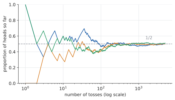
Bayesian (degree of belief). The probability of an event is a number between 0 and 1 measuring how strongly you believe it, given what you know. "70% chance of rain" means the forecaster is about as confident of rain as of drawing a red ball from an urn with 7 red and 3 blue. This reading makes sense for one-off events (tomorrow’s weather, whether a patch is buggy) and, crucially, tells you how beliefs should change when evidence arrives. That change is Bayes' theorem, coming later in Section 29.9.
The good news: both interpretations obey exactly the same rules. Whatever probability "really" is, the arithmetic in this chapter applies to it. Statisticians argue about interpretation (we return to the argument in Chapter 31); they don’t argue about the rules.
|
Probability, experiment, outcome
A random experiment is any process whose result is uncertain: rolling a die, sampling a user, running a randomized algorithm. Each possible result is an outcome. A probability is a number from 0 to 1 attached to a set of outcomes: 0 means impossible, 1 means certain. Probabilities are often written as fractions (\(\tfrac14\)), decimals (0.25) or percentages (25%); these are the same number in different clothes (Chapter 2). Odds are a different way to express the same information: odds of \(a{:}b\) in favour means probability \(\frac{a}{a + b}\). Probability \(0.2\) is odds \(1{:}4\). |
|
From gambling to mathematics
Probability theory began in 1654 with letters between Blaise Pascal and Pierre de Fermat about the "problem of points": how should the stakes of an unfinished dice game be split fairly? Gamblers had known rough odds for centuries, but nobody had a systematic method. The modern axioms, which turn probability into a branch of mathematics in its own right, were only written down in 1933, by Andrey Kolmogorov. |
29.2. Sample spaces and events
29.2.1. The problem
To say anything precise you need to pin down what can happen. "Roll two dice; what is the probability of a total of 8?" requires a list of everything that could happen, and a way to pick out the cases that count as "total of 8". Set language from Chapter 21 does exactly this.
29.2.2. Vocabulary and notation
|
Sample space and event
The sample space, written \(\Omega\) (capital Greek omega) or \(S\), is the set of all possible outcomes of an experiment. An event is a subset of the sample space: a collection of outcomes. We say "event \(A\) occurs" if the outcome that actually happens is a member of \(A\). \(P(A)\), read "the probability of \(A\)", is the probability that event \(A\) occurs. Examples. One die: \(\Omega = \{1, 2, 3, 4, 5, 6\}\); "roll is even" is the event \(\{2, 4, 6\}\). One coin tossed twice: \(\Omega = \{HH, HT, TH, TT\}\); "at least one head" is \(\{HH, HT, TH\}\). |
Because events are sets, all the set operations you know become ways of combining events. The translation table is worth memorising, because every probability word problem is written in the left-hand column and every calculation happens in the right-hand one.
| In words | Set notation | Meaning |
|---|---|---|
"not \(A\)" |
\(A^c\) (also \(\bar A\), \(A'\)) |
the complement: outcomes not in \(A\) |
"\(A\) or \(B\)" (or both) |
\(A \cup B\) |
union: outcomes in at least one |
"\(A\) and \(B\)" |
\(A \cap B\) |
intersection: outcomes in both |
"\(A\) and \(B\) can’t both happen" |
\(A \cap B = \varnothing\) |
disjoint, or mutually exclusive |
"if \(A\) happens, so does \(B\)" |
\(A \subseteq B\) |
\(A\) is a subset of \(B\) |
"something happens" / "nothing" |
\(\Omega\) / \(\varnothing\) |
the certain event / the impossible event |
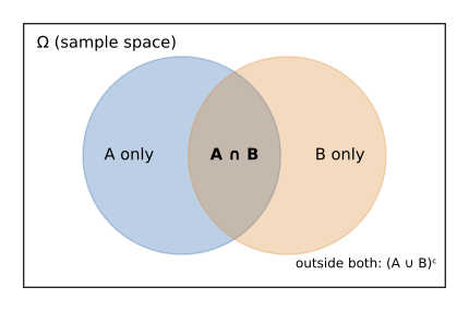
|
Complement, union, intersection, mutually exclusive
Complement \(A^c\): everything in \(\Omega\) not in \(A\). Union \(A \cup B\): "\(A\) or \(B\) or both" (mathematical "or" is always inclusive). Intersection \(A \cap B\): "both \(A\) and \(B\)". Events are mutually exclusive (or disjoint) if they share no outcomes, \(A \cap B = \varnothing\). The symbol \(\varnothing\) is the empty set. |
29.2.3. Worked example: two dice
Roll a red die and a blue die. An outcome is a pair \((r, b)\) with \(r, b \in \{1, \ldots, 6\}\), so by the product rule (Chapter 24) the sample space has \(6 \times 6 = 36\) outcomes. Picture them as a grid: Try it: Two-dice events on a grid.
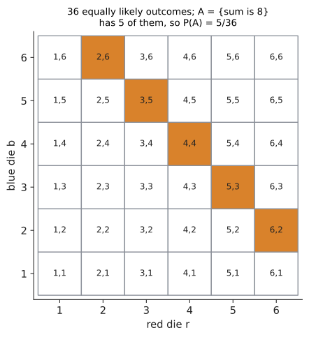
Let \(A\) = "total is 8" \(= \{(2,6), (3,5), (4,4), (5,3), (6,2)\}\), and \(D\) = "doubles" \(= \{(1,1), (2,2), \ldots, (6,6)\}\). Then
-
\(A \cap D = \{(4,4)\}\): a total of 8 and doubles;
-
\(A \cup D\) has \(5 + 6 - 1 = 10\) outcomes (subtract the one counted twice);
-
\(D^c\) is "not doubles", with \(36 - 6 = 30\) outcomes.
Notice how the question "how many outcomes?" is already doing most of the work. Probability, in the simplest setting, is counting.
|
Choosing the sample space
The same experiment can be described by different sample spaces, and a poor choice causes errors. For two dice you could take \(\Omega = \{2, 3, \ldots, 12\}\) (the possible totals). That’s a legitimate sample space, but its outcomes are not equally likely: a total of 7 can happen six ways, a total of 2 only one way. Choose a sample space whose outcomes are equally likely whenever you plan to count, and keep the dice distinguishable (red and blue) even if they look identical. |
29.3. The axioms and the basic rules
29.3.1. The problem
We need rules that every assignment of probabilities must obey, whether the numbers come from counting, from long-run frequencies or from belief. Remarkably, three rules suffice, and everything else in this chapter is derived from them.
29.3.2. The axioms
|
Kolmogorov’s axioms
A probability assigns to each event \(A\) a number \(P(A)\) such that
An axiom is a starting rule we accept without proof; everything else is derived from the axioms. |
These match intuition for frequencies. A fraction of trials can’t be negative; the fraction of trials in which something happens is 1; and if \(A\) and \(B\) never happen together, the fraction of trials in which one of them happens is the fraction for \(A\) plus the fraction for \(B\).
29.3.3. Why the other rules follow
The complement rule. \(A\) and \(A^c\) are disjoint and together make up \(\Omega\). So
and therefore \(P(A^c) = 1 - P(A)\). As special cases, \(P(\varnothing) = 1 - P(\Omega) = 0\), and since \(P(A^c) \ge 0\), \(P(A) \le 1\).
The addition rule (general). If \(A\) and \(B\) overlap, adding \(P(A) + P(B)\) counts the overlap \(A \cap B\) twice. Split the union into three disjoint pieces: "\(A\) only", "\(B\) only", "both". Then
This is inclusion–exclusion from Chapter 24, with probabilities in place of counts.
|
Complement rule and addition rule
Complement rule: \(P(A^c) = 1 - P(A)\). Addition rule: \(P(A \cup B) = P(A) + P(B) - P(A \cap B)\). If \(A\) and \(B\) are mutually exclusive, the last term is 0. Monotonicity: if \(A \subseteq B\) then \(P(A) \le P(B)\). (A more specific event can’t be more probable.) |
29.3.4. Worked examples
Example 1 (complement). What is the probability of at least one six in four rolls of a die? "At least one" has many cases (exactly one six, exactly two, …). The complement, "no sixes", is one case. Each roll avoids six in 5 of 6 ways, so by counting, \(P(\text{no sixes}) = \frac{5^4}{6^4} = \frac{625}{1296}\). Then
Slightly better than even. This was one of the bets that sparked the Pascal–Fermat letters.
Example 2 (addition rule). In a codebase, 30% of files have no tests, 20% have a lint warning, and 8% have both. What fraction of files have at least one of these problems?
So 58% of files are clean.
|
Adding probabilities that overlap
"There’s a 50% chance of rain on Saturday and 50% on Sunday, so it’s certain to rain this weekend." Wrong: the events aren’t mutually exclusive, so you must subtract the overlap. If the days were independent (Section 29.7) the chance of rain at some point would be \(1 - 0.5 \times 0.5 = 0.75\). A quick sanity check: any calculation that produces a probability above 1 has added overlapping events. |
29.3.5. Where you’d use this
-
Everyday: reading betting odds. Fractional odds of "3/1" mean you win 3 for every 1 staked, which is a fair bet only if the probability is \(1/(3 + 1) = 0.25\). For a football match priced home 6/4, draw 9/4, away 7/4, the implied probabilities are \(\tfrac{4}{10} = 0.400\), \(\tfrac{4}{13} \approx 0.308\) and \(\tfrac{4}{11} \approx 0.364\). The three outcomes are mutually exclusive and exhaustive, so the axioms say true probabilities must add to 1; these add to about 1.071. That extra 7% (the overround) is the bookmaker’s built-in margin, and the complement-and-addition rules are all you need to spot it.
-
Science: a "70% chance of rain" from a modern forecast typically means that in roughly 70% of an ensemble of slightly perturbed simulations, rain fell at your location: the frequentist reading applied to computer runs. Geneticists, epidemiologists and insurers all start from the same three axioms.
-
Computing: a classifier’s output layer (such as softmax) must produce non-negative numbers that sum to 1 across the possible labels; if your "probabilities" sum to 1.3, you have a bug, and the addition rule is the unit test. The complement rule is the standard trick for "at least one" questions in reliability and testing: "probability that at least one of 50 flaky tests fails" is \(1 - P(\text{all pass})\).
29.4. Equally likely outcomes: probability as counting
29.4.1. The problem
For fair dice, shuffled cards and random selections, every outcome in a well-chosen sample space has the same probability. Then probability reduces to counting. But the counts can be large, which is why Chapter 24 came first.
29.4.2. Why it works
Suppose \(\Omega\) has \(N\) outcomes, all equally likely, each with probability \(p\). The outcomes are disjoint and together make up \(\Omega\), so by axioms 2 and 3, \(Np = 1\) and \(p = 1/N\). An event \(A\) with \(|A|\) outcomes is the disjoint union of those outcomes, so
Input: an experiment and an event \(A\).
Steps:
-
Choose a sample space \(\Omega\) whose outcomes are equally likely. (Make objects distinguishable; decide whether order matters and stay consistent.)
-
Count \(|\Omega|\).
-
Count the outcomes in \(A\), using the same convention (ordered or unordered) as step 2.
-
If \(A\) is awkward to count, count \(A^c\) instead and use \(P(A) = 1 - P(A^c)\).
-
Compute \(P(A) = |A| / |\Omega|\) and sanity-check that it lies in \(\lbrack 0, 1]\).
Output: \(P(A)\).
29.4.3. Worked example: a poker hand
What is the probability that a 5-card hand dealt from a shuffled 52-card deck contains exactly two aces? Try it: Two aces, computed.
Step 1. Outcomes: unordered 5-card hands, all equally likely.
Step 2. \(|\Omega| = \binom{52}{5} = 2\,598\,960\).
Step 3. Build a favourable hand in two stages: choose 2 of the 4 aces, then 3 of the 48 non-aces.
Step 5. \(P(A) = \frac{103\,776}{2\,598\,960} \approx 0.0399\), about 4%.
29.4.4. Worked example: a defective batch
A batch of 20 chips has 3 defective ones. You test 4 chosen at random. What is the probability you catch at least one defective chip? Try it: Defective batch sampler.
Counting "at least one" directly means cases 1, 2 and 3. The complement, "no defectives", is one case: all 4 chosen from the 17 good chips.
Testing 4 of 20 chips gives only about a coin-flip’s chance of spotting a problem that affects 15% of the batch. Quality-control sampling plans are designed with exactly this calculation.
29.4.5. Where you’d use this
-
Everyday: lotteries. The UK Lotto draws 6 numbers from 59, so there are \(\binom{59}{6} = 45\,057\,474\) equally likely tickets and one jackpot: a probability of about 1 in 45 million per ticket. The US Powerball (5 from 69, plus 1 from 26) has \(\binom{69}{5}\times 26 = 292\,201\,338\) combinations. Buying 100 tickets a week for 50 years (260,000 tickets) still gives less than a 0.1% chance of a Powerball jackpot (\(260\,000/292\,201\,338 \approx 0.0009\)).
-
Science: in a lab, choosing 4 mice at random from 20 for a treatment group is the same counting problem as the chip batch; random assignment guarantees every group of 4 was equally likely, which is what lets the statistics in Chapter 31 work. Geneticists count equally likely allele combinations in a Punnett square.
-
Computing: the chance that a brute-force attacker guesses a random 8-character password drawn from 62 letters and digits on one try is \(1/62^8 \approx 4.6\times 10^{-15}\); password-strength meters are counting arguments. Random sampling for audits and canary deploys ("send 1% of traffic to the new version") relies on every unit being equally likely to be picked.
|
Equally likely is an assumption
\(|A|/|\Omega|\) only works if outcomes are equally likely. "Either I win the lottery or I don’t, so it’s 50–50" uses a two-outcome sample space whose outcomes are wildly unequal. Likewise, mixing ordered counts in the numerator with unordered counts in the denominator gives nonsense. A safe habit: write the words "ordered" or "unordered" next to both counts. |
29.5. Conditional probability: what conditioning means
This is the most important section of the chapter. The notation \(P(A \mid B)\) looks innocent, but the idea behind it (how a probability changes when you learn something) underlies diagnostics, spam filters, recommendation systems, A/B tests and most of machine learning.
29.5.1. The problem
Roll two dice. The probability that the total is 8 is \(5/36 \approx 0.139\). Now a friend peeks at the red die and tells you "it’s even". Should your probability for "total is 8" change? Intuitively yes: an even red die rules out some ways of getting 8 (such as \((3,5)\)) and keeps others (such as \((2,6)\)). But by how much?
29.5.2. Intuition: the information shrinks the world
Before the hint, any of 36 outcomes could be the true one. After "the red die is even", only the 18 outcomes with \(r \in \{2, 4, 6\}\) are still possible. The other 18 are ruled out. Nothing has changed about the relative chances of the outcomes that remain: they were equally likely before, and nothing in the hint favours one over another, so they are still equally likely. The new sample space is just smaller. Try it: Watch conditioning shrink the world.
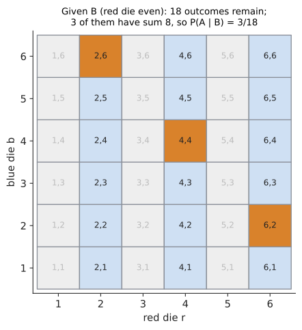
Among the 18 survivors, the totals of 8 are \((2,6)\), \((4,4)\), \((6,2)\): three of them. So the updated probability is \(3/18 = 1/6 \approx 0.167\). The hint made "total is 8" a little more likely.
That’s all conditioning is: restrict attention to the outcomes consistent with what you know, and re-measure the event as a fraction of that restricted world.
29.5.3. Why the definition looks the way it does
In the dice example the calculation was
Divide top and bottom by \(|\Omega| = 36\):
That last form doesn’t mention counting at all, so it makes sense even when outcomes aren’t equally likely. It becomes the definition.
|
Conditional probability
For events \(A\) and \(B\) with \(P(B) > 0\), the conditional probability of \(A\) given \(B\) is
\[P(A \mid B) = \frac{P(A \cap B)}{P(B)}.\]
Read the vertical bar \(\mid\) as "given". \(B\) is the conditioning event (what you know); \(A\) is the event you’re asking about. \(P(A)\), without a condition, is sometimes called the unconditional or marginal probability. Meaning: of all the probability sitting on \(B\), what fraction also lies in \(A\)? Geometrically: zoom into \(B\) and rescale it to have total probability 1. |
Read the formula as an instruction: zoom in on \(B\), then measure \(A\)'s share of it. The division by \(P(B)\) is a rescaling so that the new, smaller world has total probability 1 again. You can check that \(P(\cdot \mid B)\) satisfies all three axioms: it is a genuine probability, just on a smaller world.
29.5.4. Two-way tables: conditioning by rows and columns
Real data often arrives as a table of counts, and then conditioning is literally "restrict to a row or column". Here are 1,000 deploys of a service, classified by whether they were made on a Friday and whether they caused an incident:
| Incident | No incident | Total | |
|---|---|---|---|
Friday |
24 |
176 |
200 |
Not Friday |
40 |
760 |
800 |
Total |
64 |
936 |
1000 |
-
Unconditional: \(P(\text{incident}) = 64/1000 = 0.064\).
-
Given Friday, restrict to the Friday row: \(P(\text{incident} \mid \text{Friday}) = 24/200 = 0.12\).
-
Given not Friday: \(P(\text{incident} \mid \text{not Friday}) = 40/800 = 0.05\).
-
Reverse the question, restrict to the Incident column: \(P(\text{Friday} \mid \text{incident}) = 24/64 = 0.375\).
Check the definition gives the same thing: \(P(\text{incident} \cap \text{Friday}) / P(\text{Friday}) = 0.024 / 0.2 = 0.12\). ✓
Friday deploys are more than twice as likely to cause incidents. (Whether Fridays cause incidents is a different question; see correlation versus causation in Chapter 31.)
Input: events \(A\) and \(B\), and a way to find probabilities (counts, a table, or given numbers).
Steps:
-
Identify which event is known (it goes after the bar) and which is asked about. Rewrite the question as "of the cases where [known], what fraction have [asked]?"
-
Find \(P(B)\), or count \(|B|\) in a table or equally-likely sample space.
-
Find \(P(A \cap B)\), or count \(|A \cap B|\).
-
Divide: \(P(A \mid B) = P(A \cap B)/P(B)\).
Output: \(P(A \mid B)\).
29.5.5. Worked example: two children
A family has two children. Assume each child is independently a boy or a girl with probability 1/2. Given that at least one is a girl, what is the probability that both are girls?
Sample space (ordered by birth, so equally likely): \(\{BB, BG, GB, GG\}\).
-
Known: \(B\) = "at least one girl" \(= \{BG, GB, GG\}\). Asked: \(A\) = "both girls" \(= \{GG\}\).
-
\(P(B) = 3/4\).
-
\(A \cap B = \{GG\}\), so \(P(A \cap B) = 1/4\).
-
\(P(A \mid B) = \dfrac{1/4}{3/4} = \dfrac13\).
Not 1/2, which is most people’s first answer. The information "at least one girl" removes only \(BB\), leaving three equally likely worlds, and only one of them is \(GG\). If instead you’re told "the elder child is a girl", the world shrinks to \(\{GB, GG\}\) and the answer is 1/2. Different information, different restricted world, different answer. Conditioning is sensitive to exactly what you learned.
29.5.6. Where you’d use this
-
Everyday: conditional probabilities are what you actually want from your own records. If over a year you were late on 9 of 30 rainy days but only 20 of 200 dry ones, then \(P(\text{late} \mid \text{rain}) = 0.3\) while \(P(\text{late} \mid \text{dry}) = 0.1\): leave earlier when it rains. Car-insurance premiums are set the same way, from the claim rate given the driver’s age band and postcode.
-
Science and medicine: survival rates, side-effect rates and test accuracy are all conditional ("5-year survival given diagnosis at stage 1"), and quoting one without its condition is the most common way statistics mislead.
-
Computing: "customers who bought this also bought". Suppose 2,000 of 10,000 supermarket baskets contain pasta, 800 of those also contain parmesan, and 500 baskets in total contain parmesan. Then \(P(\text{parmesan} \mid \text{pasta}) = 800/2000 = 0.4\), against \(P(\text{parmesan}) = 500/10\,000 = 0.05\) overall: buying pasta makes parmesan 8 times as likely. Association-rule mining calls 0.4 the rule’s confidence and the factor 8 its lift; recommendation engines and shelf layouts are built from such numbers.
|
Confusing P(A | B) with P(B | A)
\(P(\text{incident} \mid \text{Friday}) = 0.12\) but \(P(\text{Friday} \mid \text{incident}) = 0.375\). These are different questions, divided by different totals (a row versus a column). Swapping them is called the confusion of the inverse, and in court it’s the prosecutor’s fallacy: "If the defendant were innocent, there’s only a 1 in a million chance the DNA would match, so there’s only a 1 in a million chance he’s innocent." The first probability is \(P(\text{match} \mid \text{innocent})\); the jury needs \(P(\text{innocent} \mid \text{match})\), which depends on how many other people could have matched. In a city of 10 million, around 10 innocent people would match. Bayes' theorem (below) is the tool for turning one into the other. |
29.6. The multiplication rule and tree diagrams
29.6.1. The problem
Often you know conditional probabilities and want a joint one. A bag holds 5 red and 3 blue marbles. Draw two without replacement. What’s the chance both are red? The second draw depends on the first.
29.6.2. Why it works
Multiply both sides of the definition of conditional probability by \(P(B)\):
This is the multiplication rule: the chance that both happen is the chance that the first happens times the chance the second happens given the first. For three events it chains: \(P(A \cap B \cap C) = P(A)\,P(B \mid A)\,P(C \mid A \cap B)\).
For the marbles, with \(R_1\) = "first is red", \(R_2\) = "second is red":
Check by counting: \(\binom52 / \binom82 = 10/28 = 5/14\). ✓ Two different methods, same answer.
29.6.3. Tree diagrams
A tree diagram draws the multiplication rule. Each level is a stage of the experiment; each branch carries the conditional probability of that branch given the path so far. The probability of a complete path is the product of the probabilities along it, and the probability of an event is the sum of the paths that make it up.
Input: a multi-stage experiment.
Steps:
-
Draw one level per stage. At each node, draw a branch for every possible result of the next stage.
-
Label each branch with its probability conditional on the path leading to it. Branches leaving any node must sum to 1.
-
Multiply along each root-to-leaf path to get the probability of that path (multiplication rule).
-
Add the probabilities of all paths in your event (addition rule: paths are disjoint).
Output: the probability of the event.
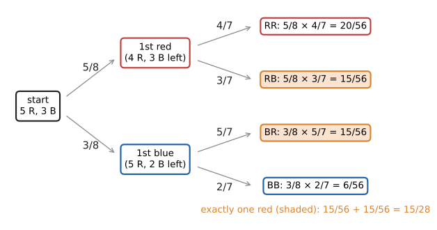
For the marbles, "exactly one red" consists of two paths, RB and BR:
And \(P(\text{BB}) = \frac38 \times \frac27 = \frac{6}{56}\). The four paths sum to \(\frac{20 + 15 + 15 + 6}{56} = 1\). ✓
29.6.4. Where you’d use this
A tree diagram is the right tool whenever an outcome happens in stages. Everyday: the chance of being dealt two aces from a shuffled deck is \(\tfrac{4}{52}\times\tfrac{3}{51} = \tfrac{12}{2652} = \tfrac{1}{221}\), about 0.45%, which is why poker players treat it as a once-in-an-evening event. Science: a diagnostic pathway (screen, then confirm, then treat) is a tree, as is a multi-stage chemical synthesis whose overall yield is the product of the stage yields. Computing: a funnel in product analytics (visit, then sign up, then pay) multiplies conditional conversion rates; 20% sign up and 10% of those pay gives \(0.2\times 0.1 = 2\%\) of visitors paying.
29.7. Independence
29.7.1. The problem
Sometimes learning \(B\) tells you nothing about \(A\). Knowing the red die shows 3 says nothing about the blue die. Knowing it rained in Tokyo says nothing about a coin toss in London. We need a word for this, because it simplifies calculations enormously, and because wrongly assuming it causes some of the worst mistakes in applied probability.
29.7.2. Definition and intuition
\(A\) and \(B\) are independent if conditioning on \(B\) doesn’t change the probability of \(A\): \(P(A \mid B) = P(A)\). Substituting the definition of conditional probability and multiplying by \(P(B)\) gives the symmetric form usually taken as the definition.
|
Independent events
Events \(A\) and \(B\) are independent if
\[P(A \cap B) = P(A)\,P(B).\]
Equivalently (when \(P(B) > 0\)), \(P(A \mid B) = P(A)\): knowing \(B\) happened doesn’t change the probability of \(A\). Events that aren’t independent are dependent. Several events \(A_1, \ldots, A_n\) are mutually independent if the product rule holds for every sub-collection, e.g. \(P(A_1 \cap A_2 \cap A_3) = P(A_1)P(A_2)P(A_3)\). |
In the dice example, "total is 8" and "red is even" are dependent: \(P(A \mid B) = 1/6 \ne 5/36 = P(A)\). In the deploy table, "incident" and "Friday" are dependent: \(0.12 \ne 0.064\).
By contrast, let \(C\) = "total is 7" and \(B\) = "red is even". The totals of 7 with even red are \((2,5), (4,3), (6,1)\), so \(P(C \mid B) = 3/18 = 1/6\), and \(P(C) = 6/36 = 1/6\). Equal, so \(C\) and \(B\) are independent. Independence is a numerical fact, not always something you can see in advance.
29.7.3. Applications: reliability
Independence is how engineers compute reliability. Suppose each of three servers is up 99% of the time, independently. Try it: Build your own reliability diagram; Three replicas in parallel; Three servers in series.
-
In series (the request needs all three, e.g. a chain of microservices): \(P(\text{all up}) = 0.99^3 \approx 0.970\). Chaining services multiplies their unreliability.
-
In parallel (any one suffices, e.g. redundant replicas): use the complement. \(P(\text{all down}) = 0.01^3 = 10^{-6}\), so \(P(\text{at least one up}) = 1 - 10^{-6} = 0.999999\): "six nines".
29.7.4. More applications: genetics and everyday risk
-
Science: inheritance. Cystic fibrosis is recessive: a child is affected only if it inherits the faulty allele from both parents. If both parents are carriers, each child independently has probability \(\tfrac12\times\tfrac12 = \tfrac14\) of being affected. For a family of three children, \(P(\text{none affected}) = (\tfrac34)^3 = \tfrac{27}{64}\), so \(P(\text{at least one affected}) = 1 - \tfrac{27}{64} = \tfrac{37}{64} \approx 0.58\). Genetic counsellors give exactly these numbers. Mendel’s peas worked because separate genes are (mostly) inherited independently.
-
Everyday: a thief with your phone gets 3 guesses at a random 4-digit PIN: \(3/10\,000 = 0.03\%\). Those guesses aren’t independent trials (a sensible thief never repeats a guess), which is why the answer is exactly \(3/10\,000\) rather than \(1 - 0.9999^3\); the two differ only in the eighth decimal place here, but the habit of asking "independent or not?" is the point.
-
Engineering: twin-engine aircraft, dual brake circuits in cars and backup generators in hospitals are the "parallel" calculation above, and the reason regulators insist the redundant parts share as little as possible (separate fuel lines, separate wiring) is precisely to keep failures independent.
|
Independent is not the same as disjoint
Mutually exclusive events with positive probability are always dependent: if \(A\) and \(B\) are disjoint and \(B\) happens, \(A\) certainly didn’t, so \(P(A \mid B) = 0 \ne P(A)\). "Can’t happen together" and "don’t influence each other" are opposite ideas, not the same one. The other classic trap is assuming independence. The replica calculation above fails badly if the three servers share a power supply, a network switch or a buggy config push: then failures are correlated and \(P(\text{all down})\) might be \(10^{-3}\), not \(10^{-6}\). The 2008 financial crisis was, in part, a correlated-failure miscalculation: mortgage defaults were modelled as nearly independent, and they weren’t. |
|
The gambler’s fallacy
On 18 August 1913, at the casino in Monte Carlo, a roulette wheel came up black 26 times in a row. Gamblers lost millions betting on red, reasoning that red was "due". But successive spins are independent: the wheel has no memory, and after 25 blacks the next spin is still red with probability 18/37. Believing that independent events "balance out" in the short run is the gambler’s fallacy. The law of large numbers (Chapter 30) says the proportion evens out over the long run, but it does so by swamping early streaks with many later spins, not by correcting them. |
29.8. The law of total probability
29.8.1. The problem
A factory has two production lines. Line 1 makes 60% of the chips and 2% of its chips are defective; line 2 makes 40% and 5% of its chips are defective. What fraction of all chips is defective? You know the defect rate conditional on each line; you want the overall rate.
29.8.2. Why it works
The lines split the sample space into disjoint pieces that cover everything. Every defective chip came from exactly one line, so
The overall defect rate is 3.2%, a weighted average of the line rates with weights equal to each line’s share.
|
Partition and the law of total probability
Events \(B_1, B_2, \ldots, B_n\) form a partition of \(\Omega\) if they are mutually exclusive and together cover \(\Omega\): every outcome lies in exactly one \(B_i\). The law of total probability says, for any event \(A\),
\[P(A) = \sum_{i=1}^{n} P(B_i)\,P(A \mid B_i).\]
Here \(\sum_{i=1}^{n}\) ("sigma") means "add the following expression for \(i = 1, 2, \ldots, n\)". In a tree diagram, this is "add up every path that ends in \(A\)". Simplest case: \(P(A) = P(B)P(A \mid B) + P(B^c)P(A \mid B^c)\). |
The law is a "divide and conquer" strategy: when \(P(A)\) is hard, split the world into cases where it’s easy, and recombine with weights.
29.8.3. Where you’d use this
-
Everyday: you take the train 70% of the time and are late 10% of those days; you take the bus otherwise and are late 25% of those days. Then \(P(\text{late}) = 0.7\times 0.10 + 0.3\times 0.25 = 0.07 + 0.075 = 0.145\): about one day in seven.
-
Medicine: what fraction of everyone tested will see a positive result? Split by whether they have the disease: \(0.01\times 0.99 + 0.99\times 0.05 = 0.0099 + 0.0495 = 0.0594\), so 5.94% of tests come back positive. That denominator is exactly the 594 positives out of 10,000 in the next section, where it becomes the bottom line of Bayes' theorem.
-
Computing: the overall error rate of a service running in several regions is the traffic-weighted average of the regional error rates, and the overall false-positive rate of a classifier on a mixed dataset is the weighted average over its sub-populations. When an aggregate number looks surprising (a "better" model that is worse in every subgroup, Simpson’s paradox, Chapter 31), the cause is almost always a change in the weights.
29.9. Bayes' theorem
29.9.1. The problem
A disease affects 1% of people. A test for it has a 99% true-positive rate (if you have the disease, it’s positive 99% of the time) and a 5% false-positive rate (if you don’t, it’s still positive 5% of the time). You test positive. What is the probability you have the disease? Try it: The test as 1,000 people.
Most people, including, in published studies, most doctors, answer something like 95% or 99%. The true answer is about 17%. Let’s see why, two ways.
29.9.2. Intuition: natural frequencies
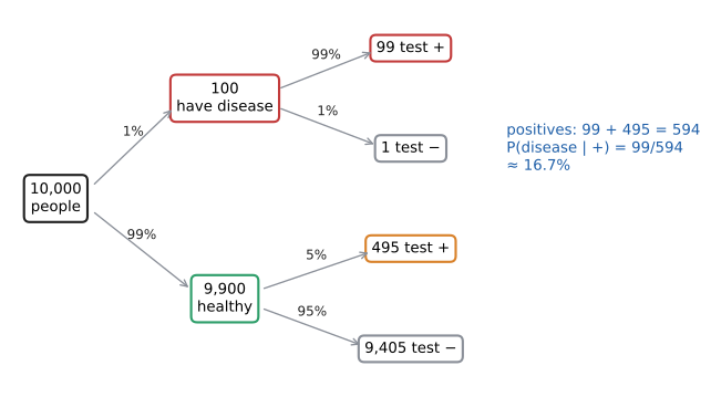
Imagine 10,000 people taking the test. Replace each probability with a count: Try it: Medical test as frequencies.
-
1% have the disease: 100 people. 9,900 don’t.
-
Of the 100 with the disease, 99% test positive: 99 people.
-
Of the 9,900 healthy people, 5% test positive anyway: 495 people.
-
Total positives: \(99 + 495 = 594\).
You are one of the 594 positives. Of those, 99 are sick. So
The test is good, but the disease is rare. Healthy people are 99 times as numerous as sick ones, so even a small false-positive rate among the healthy produces five times as many false alarms as true alarms. Conditioning on "positive" restricts you to the 594 positives, and in that restricted world, sick people are a minority. This is the base-rate fallacy: ignoring how common the condition was in the first place (its base rate or prior).
29.9.3. Why it works: deriving Bayes' theorem
Nothing new is needed; Bayes' theorem is the definition of conditional probability, used twice. The multiplication rule gives \(P(A \cap B)\) two ways:
Set them equal and divide by \(P(B)\):
The denominator \(P(B)\) is usually not given directly, so expand it with the law of total probability over \(A\) and \(A^c\):
That’s Bayes' theorem. It "inverts" a conditional probability: from \(P(B \mid A)\) (which a lab can measure: how does the test behave on sick people?) to \(P(A \mid B)\) (which the patient wants: given my result, am I sick?).
|
Bayes' theorem: prior, likelihood, posterior
\[\underbrace{P(H \mid E)}_{\text{posterior}} = \frac{\overbrace{P(E \mid H)}^{\text{likelihood}}\;\overbrace{P(H)}^{\text{prior}}}{\underbrace{P(E)}_{\text{evidence}}}\]
\(H\) is a hypothesis (has the disease), \(E\) the evidence (tested positive).
For tests: sensitivity = \(P( + \mid \text{disease})\) (true-positive rate); specificity = \(P(- \mid \text{healthy})\); false-positive rate = \(1 -\) specificity. |
29.9.4. Worked example: the formula, every step
With \(D\) = disease and \({ + }\) = positive test: \(P(D) = 0.01\), \(P(D^c) = 0.99\), \(P( + \mid D) = 0.99\), \(P( + \mid D^c) = 0.05\).
Same answer as the tree, because the tree is the formula: 99 is \(10\,000 \times 0.0099\) and 594 is \(10\,000 \times 0.0594\).
What if you take a second, independent test and it’s also positive? Use the posterior as the new prior: \(P(D) = 1/6\). Try it: The second positive test; Add a second test.
Two positives take you from 1% to about 80%. Evidence accumulates; this is why doctors confirm a positive screening test with a second, different test (which also helps ensure the "independent" assumption is reasonable).
Input: prior \(P(H)\), likelihoods \(P(E \mid H)\) and \(P(E \mid H^c)\).
Steps:
-
Compute the two joint probabilities: \(a = P(E \mid H)P(H)\) (evidence and hypothesis true) and \(b = P(E \mid H^c)\,(1 - P(H))\) (evidence and hypothesis false).
-
The evidence probability is \(P(E) = a + b\).
-
The posterior is \(P(H \mid E) = a/(a + b)\).
-
For further independent evidence, repeat with the posterior as the new prior.
Output: the posterior \(P(H \mid E)\).
Check: draw the natural-frequency tree for 10,000 (or 100,000) cases; the leaf counts should be \(10\,000a\) and \(10\,000b\).
import random

def posterior(prior, sensitivity, false_pos_rate):
    """P(disease | positive test) by Bayes' theorem."""
    p_pos = sensitivity * prior + false_pos_rate * (1 - prior)  # total probability
    return sensitivity * prior / p_pos

print(round(posterior(0.01, 0.99, 0.05), 4))

# Check by simulating a million patients
random.seed(2)
sick_and_pos = pos = 0
for _ in range(1_000_000):
    sick = random.random() < 0.01
    if sick:
        positive = random.random() < 0.99
    else:
        positive = random.random() < 0.05
    if positive:
        pos += 1
        sick_and_pos += sick
print(round(sick_and_pos / pos, 4))
0.1667 0.166
The simulation does exactly what conditioning means: it throws away every simulated patient who tested negative and asks what fraction of the rest are sick.
29.9.5. Alternative approach: the odds form
Bayes' theorem is even simpler in odds. Divide the Bayes formula for \(H\) by the one for \(H^c\); the awkward denominator \(P(E)\) cancels:
For the test: prior odds \(1{:}99\); likelihood ratio \(0.99/0.05 = 19.8\); posterior odds \(19.8{:}99 = 1{:}5\), i.e. probability \(1/6\). ✓ A second positive multiplies by 19.8 again: \(19.8{:}5 \approx 4{:}1\), about 80%. ✓
29.9.6. Choosing a method
-
Natural frequency tree: best for explaining to anyone (including yourself at 2 a.m.), and best for catching errors. Use it first whenever the numbers are percentages.
-
Formula: best when you need a general expression or code.
-
Odds form: best for sequential evidence (just keep multiplying by likelihood ratios) and for quick mental estimates. It is the form used by naive Bayes classifiers.
-
Simulation: best as an independent check, and for problems too messy for algebra.
29.9.7. Where you’d use this
-
Everyday: any time a "pretty accurate" signal fires for a rare event: a smoke alarm, a fraud alert on your card, a home pregnancy or COVID test, a "your account has been compromised" email. The base rate of the event matters as much as the accuracy of the signal, and the natural-frequency tree tells you how much to trust the alarm.
-
Science and engineering: Bayesian search theory updates a map of where a lost object might be after each unsuccessful search, multiplying the probability of each search area by the chance the search would have missed it there. It located the wreck of the submarine USS Scorpion in 1968, and in 2011 a Bayesian reanalysis of the earlier, unsuccessful searches pointed searchers to the wreckage of Air France 447 on the floor of the Atlantic, found within about a week of resuming. Self-driving cars and phone GPS fuse noisy sensor readings with the Kalman filter, which is Bayes' theorem applied repeatedly to continuous quantities.
-
Computing: spam filtering (below), A/B testing that reports "probability variant B is better", and probabilistic programming all apply this one formula.
|
Where Bayes goes wrong in practice
|
|
Reverend Bayes and Mr Price
Thomas Bayes, an English Presbyterian minister, never published his theorem. After his death in 1761 his friend Richard Price found the essay among his papers, edited it and presented it to the Royal Society in 1763. Pierre-Simon Laplace independently discovered the general form and used it for decades to analyse astronomical and census data. For much of the 20th century "Bayesian" methods were unfashionable; cheap computing brought them back, and today Bayesian updating runs inside spam filters, robot localisation, medical decision aids and search-and-rescue planning. |
|
Bayes slider
Three sliders (prevalence, sensitivity, false-positive rate) drive a live natural-frequency tree and an "icon array" of 1,000 people, colouring true positives, false positives, true negatives and false negatives. Watch the posterior collapse as you slide prevalence from 50% down to 0.1%, and see how much specificity you’d need to make a rare-disease screen useful. A second mode adds a second, independent test. Try it: Slide the prevalence · Bayes slider lab |
29.10. Two famous puzzles
29.10.1. The Monty Hall problem
In a game show there are three doors: a car behind one, goats behind the other two. You pick a door, say door 1. The host, who knows where the car is, opens one of the other doors to reveal a goat (if both hide goats he picks one at random), and offers you the chance to switch to the remaining closed door. Should you? Try it: Play Monty Hall.
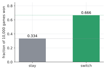
The almost universal first reaction is "two doors left, so it’s 50–50; switching doesn’t matter". That’s wrong: switching wins with probability 2/3.
Argument 1: what your first pick tells you. Your first pick is right with probability 1/3 and wrong with probability 2/3. The host’s action never changes that: he can always open a goat door, whatever you picked. If you were right (prob. 1/3), switching loses. If you were wrong (prob. 2/3), the host has been forced to reveal the other goat, so the remaining door must hide the car, and switching wins. Switching wins exactly when your first pick was wrong: probability 2/3.
Argument 2: Bayes. Let \(C_i\) = "car behind door \(i\)" and \(O_3\) = "host opens door 3". You picked door 1. Priors: \(P(C_i) = 1/3\). Likelihoods of the host’s action:
-
if the car is behind 1, the host chooses 2 or 3 at random: \(P(O_3 \mid C_1) = 1/2\);
-
if the car is behind 2, the host must open 3: \(P(O_3 \mid C_2) = 1\);
-
if the car is behind 3, the host can’t open 3: \(P(O_3 \mid C_3) = 0\).
The host’s choice carries information because it is constrained: he will never open the car’s door. The intuition "50–50" would be right if the host opened a door at random and happened to reveal a goat; that’s a different experiment (try it in the simulation below).
import random

def play(switch, rng):
    car = rng.randrange(3)
    pick = rng.randrange(3)
    # host opens a door that is neither the pick nor the car
    opened = rng.choice([d for d in range(3) if d != pick and d != car])
    if switch:
        pick = next(d for d in range(3) if d != pick and d != opened)
    return pick == car

rng = random.Random(3)
n = 100_000
print("stay  :", sum(play(False, rng) for _ in range(n)) / n)
print("switch:", sum(play(True, rng) for _ in range(n)) / n)
stay : 0.33329 switch: 0.66607
|
Ten thousand letters
When Marilyn vos Savant gave the "switch" answer in Parade magazine in 1990, she received around 10,000 letters, nearly a thousand of them from people with PhDs, many telling her she was wrong. The mathematician Paul Erdős reportedly remained unconvinced until he watched a computer simulation. Simulation is a legitimate way to settle a probability argument, and a humbling one. |
29.10.2. The birthday problem
In Chapter 24 you counted the ways for \(n\) people to have distinct birthdays. Now read the same calculation as a chain of conditional probabilities. Ignore leap years and assume all 365 days equally likely. Add people one at a time. Given that the first \(k\) people all have different birthdays, person \(k + 1\) avoids all of them with probability \((365 - k)/365\). By the multiplication rule,
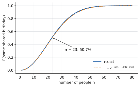
For \(n = 23\) this gives \(0.507\): better than even. The surprise is resolved by counting pairs, not people: 23 people make \(\binom{23}{2} = 253\) pairs, and each pair matches with probability \(1/365\). Try it: Birthday problem calculator.
An approximation (optional, uses \(e\) from Chapter 12). For small \(x\), \(1 - x \approx e^{-x}\). Each factor is \(1 - k/365 \approx e^{-k/365}\), so the product is about
The exponent \(n(n-1)/2\) is the number of pairs. For \(n = 23\), \(1 - e^{-253/365} \approx 0.500\). Setting the probability to 1/2 and solving gives \(n \approx 1.18\sqrt{365} \approx 22.5\). In general, with \(N\) equally likely values, a repeat becomes likely after about \(\sqrt{N}\) draws.
import math, random

def p_shared(n, days=365):
    p_distinct = 1.0
    for k in range(n):
        p_distinct *= (days - k) / days
    return 1 - p_distinct

def simulate(n, days=365, trials=100_000, seed=4):
    rng = random.Random(seed)
    hits = 0
    for _ in range(trials):
        seen = set()
        for _ in range(n):
            b = rng.randrange(days)
            if b in seen:
                hits += 1
                break
            seen.add(b)
    return hits / trials

for n in (10, 23, 50):
    approx = 1 - math.exp(-n * (n - 1) / (2 * 365))
    print(n, round(p_shared(n), 4), round(approx, 4), simulate(n))
10 0.1169 0.116 0.1175 23 0.5073 0.5 0.50933 50 0.9704 0.9651 0.97013
Try it: Birthday bound for hashes.
29.11. Probability at work in computing
29.11.1. Randomized algorithms
The problem. Quicksort picks a pivot, partitions the array into elements smaller and larger than the pivot, and recurses. If the pivot is always the first element, a sorted input makes every partition maximally lopsided, and quicksort takes about \(n^2/2\) comparisons instead of about \(n \log n\). An adversary (or just unlucky real-world data, which is often nearly sorted) can always find the bad input for a fixed rule.
The idea. Choose the pivot uniformly at random. Now there are no bad inputs, only bad luck, and bad luck is rare: for every input, the expected number of comparisons is about \(2n \ln n \approx 1.39\, n \log_2 n\). (The derivation uses linearity of expectation; see Chapter 30.) The probability shifts from the input, which you don’t control, to the coin flips, which you do.
|
Randomized algorithm, Las Vegas, Monte Carlo
A randomized algorithm makes random choices during its execution. Two families:
Mnemonic: in Las Vegas you always leave with a (correct) answer but you don’t know how long you’ll be there; in Monte Carlo you leave on time but might have lost. |
A Monte Carlo example: Freivalds' algorithm. Given \(n \times n\) matrices \(A\), \(B\), \(C\) (Chapter 27), is \(AB = C\)? Multiplying out costs about \(n^3\) operations. Instead, pick a random vector \(r\) of 0s and 1s and check whether \(A(Br) = Cr\): three matrix–vector products, about \(3n^2\) operations. If \(AB = C\), the check always passes. If \(AB \ne C\), one can show it fails with probability at least 1/2. After 20 independent rounds that all pass, the chance of being fooled is at most \(2^{-20} \approx 10^{-6}\), by independence of the rounds.
import random

def matmul_vec(M, v):
    return [sum(a * b for a, b in zip(row, v)) for row in M]

def freivalds(A, B, C, rounds=20, rng=random):
    """Monte Carlo check that A @ B == C. Never wrong when it says False."""
    n = len(A)
    for _ in range(rounds):
        r = [rng.randint(0, 1) for _ in range(n)]
        if matmul_vec(A, matmul_vec(B, r)) != matmul_vec(C, r):
            return False          # definitely not equal
    return True                   # equal, with error prob <= 2**-rounds

A = [[1, 2], [3, 4]]
B = [[5, 6], [7, 8]]
good = [[19, 22], [43, 50]]
bad = [[19, 22], [43, 51]]
random.seed(5)
print(freivalds(A, B, good), freivalds(A, B, bad))
True False
Choosing between them. Prefer Las Vegas when a wrong answer is unacceptable and you can tolerate variable latency (sorting, hashing with retries). Prefer Monte Carlo when a fixed time budget matters and you can make the error probability smaller than, say, the chance of a cosmic-ray bit flip (primality testing in cryptography, as in Chapter 23, is the classic case).
29.11.2. A naive Bayes spam filter
The problem. Decide whether an incoming message is spam from the words it contains. You have labelled history, from which you can measure how often each word appears in spam and in legitimate mail ("ham"). This is the medical test again, with words as test results. Try it: Train the spam filter.
The model. Let \(S\) = "spam". For a message containing words \(w_1, \ldots, w_k\), Bayes gives
Estimating \(P(w_1, \ldots, w_k \mid S)\) for every combination of words is hopeless: there are too many combinations. The naive assumption is that words are conditionally independent given the class:
It’s obviously false ("Nigerian" and "prince" are not independent in spam), but the classifier only needs to rank spam above ham, and it does that well. Compute an unnormalized score for each class, then divide by their sum (the law of total probability, in disguise).
Worked example. Training data: 4 spam and 6 ham messages.
| Class | Messages |
|---|---|
spam |
"free money now", "free offer meeting", "win free prize", "cheap money offer" |
ham |
"meeting at noon", "project meeting notes", "free for lunch", "meeting moved", "code review today", "lunch plans" |
Estimates (fraction of messages in the class that contain the word):
A new message contains "free" and "meeting". Scores:
Mildly spammy. "Free" alone would give \(0.3/(0.3 + 0.1) = 0.75\); the word "meeting" pulled it back towards ham.
spam = ["free money now", "free offer meeting", "win free prize",
        "cheap money offer"]
ham = ["meeting at noon", "project meeting notes", "free for lunch",
       "meeting moved", "code review today", "lunch plans"]

def doc_freq(docs, word, alpha=0):
    """Fraction of docs containing word (alpha = add-alpha smoothing)."""
    hits = sum(word in d.split() for d in docs)
    return (hits + alpha) / (len(docs) + 2 * alpha)

def p_spam(words, alpha=0):
    n = len(spam) + len(ham)
    score_s = len(spam) / n
    score_h = len(ham) / n
    for w in words:
        score_s *= doc_freq(spam, w, alpha)
        score_h *= doc_freq(ham, w, alpha)
    return score_s / (score_s + score_h)

print(round(p_spam(["free", "meeting"]), 3))
print(round(p_spam(["free"]), 3))
print(round(p_spam(["prize"]), 3), round(p_spam(["prize", "meeting"]), 3))
print(round(p_spam(["prize", "meeting"], alpha=1), 3))
0.6 0.75 1.0 1.0 0.542
|
The zero-count problem
"prize" never appears in the ham training set, so \(P(\text{prize} \mid H) = 0\), the ham score is 0 whatever else the message says, and the filter is certain it’s spam, even for "prize" plus "meeting". This is the "prior of 0" failure from the Bayes Watch out, in another form. The standard fix is Laplace (add-one) smoothing: pretend every word was seen once more in each class, and adjust the denominators so probabilities still sum to 1 (in our binary "contains the word or not" model, add 2 to the denominator). With smoothing the same message scores 0.542. Real filters also add logarithms of probabilities instead of multiplying them, to avoid floating-point underflow when multiplying hundreds of small numbers (Chapter 12, Chapter 32). |
29.11.3. Bloom filters: designing for a false-positive rate
The problem. You want a compact set that answers "have I seen this URL / key / username before?" using far less memory than storing the items. You can accept occasional false positives ("probably yes" when the answer is no) but never false negatives. Databases use this to skip disk reads; browsers once used it to check URLs against malware lists. Try it: Bloom filter explorer.
The data structure. A Bloom filter is an array of \(m\) bits, all 0, plus \(k\) hash functions. To add an item, hash it \(k\) ways and set those \(k\) bits to 1. To query, check the \(k\) bits: if any is 0, the item was definitely never added; if all are 1, it probably was.
The probability. Insert \(n\) items. Treat each hash as a uniformly random, independent position. Focus on one particular bit. (The last step uses \((1 - \tfrac1m)^m \approx e^{-1}\), an optional fact from Chapter 12.)
So a bit is 1 with probability about \(1 - e^{-kn/m}\). A query for a new item gives a false positive when all \(k\) of its bits happen to be 1. Treating those as independent:
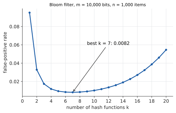
There’s a tradeoff in \(k\): more hashes give each query more chances to find a 0, but also fill the array faster. The best choice turns out to be \(k \approx (m/n)\ln 2\). With \(m/n = 10\) bits per item, \(k \approx 6.9\), and the false-positive rate is under 1%.
import hashlib, math, random

class BloomFilter:
    def __init__(self, m, k):
        self.m, self.k = m, k
        self.bits = bytearray(m)          # one byte per bit, for clarity

    def _positions(self, item):
        for i in range(self.k):
            h = hashlib.sha256(f"{i}:{item}".encode()).digest()
            yield int.from_bytes(h[:8], "big") % self.m

    def add(self, item):
        for p in self._positions(item):
            self.bits[p] = 1

    def might_contain(self, item):
        return all(self.bits[p] for p in self._positions(item))

m, n, k = 10_000, 1_000, 7
bf = BloomFilter(m, k)
for i in range(n):
    bf.add(f"user{i}")

tests = 20_000
false_pos = sum(bf.might_contain(f"other{j}") for j in range(tests))
print("measured :", false_pos / tests)
print("predicted:", round((1 - math.exp(-k * n / m)) ** k, 5))
measured : 0.00815 predicted: 0.00819
The independence assumptions in the derivation are not exactly true, but measurement agrees with prediction to within the noise. That’s a pattern worth noticing: a model built on slightly false assumptions can still be extremely useful, provided you check it.
|
Simulate before you believe
A sandbox with a two-dice grid where you click cells to define events \(A\) and \(B\). The lab shades \(A \cap B\), displays \(P(A)\), \(P(B)\), \(P(A \mid B)\) and \(P(B \mid A)\), flags whether the events are independent, and animates "conditioning" as the non-\(B\) cells fading away. A second panel runs Monty Hall with a "host knows" / "host is random" toggle, so you can see the 2/3 answer turn into 1/2 when the host stops carrying information. |
29.12. Interactive tools
Browser tools on the companion website that go with this chapter. Each example link in the chapter opens one of them with that example already set up.
29.13. Exercises
-
(Recognition) Translate into set notation and say whether each pair is mutually exclusive: (a) "a card is a heart" and "a card is a king"; (b) "a die shows an even number" and "a die shows 5"; (c) "a request times out" and "a request returns 200 OK".
-
(Recognition) Which of these is \(P(A \mid B)\) and which \(P(B \mid A)\), with \(A\) = "email is spam", \(B\) = "email contains a link"? (i) "Of spam emails, 90% contain a link." (ii) "Of emails with links, 30% are spam."
-
(Application) Two dice are rolled. Find (a) \(P(\text{total} \ge 10)\); (b) \(P(\text{at least one six})\); (c) \(P(\text{at least one six} \mid \text{total} \ge 10)\). Try it: Two dice distribution; Check exercise 3 on the grid.
-
(Application) A drawer holds 4 black and 6 white socks. You pull two at random. Find the probability they match, using a tree diagram; check by counting.
-
(Application) \(P(A) = 0.5\), \(P(B) = 0.4\), \(P(A \cup B) = 0.7\). Find \(P(A \cap B)\) and \(P(A \mid B)\). Are \(A\) and \(B\) independent?
-
(Application) 2% of transactions are fraudulent. A fraud model flags 95% of fraudulent transactions and 3% of legitimate ones. What fraction of flagged transactions are actually fraudulent? Draw the natural-frequency tree for 100,000 transactions. Try it: Fraud flags tree.
-
(Problem solving) Show that if \(A\) and \(B\) are independent, so are \(A\) and \(B^c\).
-
(Problem solving) A Monty Hall variant has 4 doors; the host knowingly opens 2 goat doors from the 3 you didn’t pick, and offers a switch to the one remaining. What is the probability of winning by switching? Try it: Monty Hall with 100 doors; Monty Hall with 4 doors.
-
(Problem solving, CS) A Monte Carlo primality test declares a composite number "probably prime" with probability at most 1/4 per round, independently. How many rounds guarantee an error probability below \(10^{-12}\)?
-
(Problem solving, CS) A Bloom filter has \(m = 8 \times 10^6\) bits and will hold \(n = 10^6\) items. Find the optimal \(k\) (nearest integer) and the resulting false-positive rate. Try it: Check your Bloom design.
Answers
-
(a) \(H \cap K\) is {king of hearts}, not empty: not mutually exclusive. (b) \(\{2,4,6\} \cap \{5\} = \varnothing\): mutually exclusive. (c) Mutually exclusive (assuming a timed-out request returns no status).
-
(i) is \(P(B \mid A) = 0.9\) (restricted to spam). (ii) is \(P(A \mid B) = 0.3\) (restricted to emails with links).
-
(a) Totals ≥ 10: (4,6),(5,5),(6,4),(5,6),(6,5),(6,6): 6 outcomes, \(6/36 = 1/6\). (b) Complement: \(1 - 25/36 = 11/36\). (c) Restrict to the 6 outcomes in (a); those with a six: (4,6),(6,4),(5,6),(6,5),(6,6) = 5. So \(5/6\).
-
Tree: \(P(BB) = \frac4{10} \cdot \frac39 = \frac{12}{90}\), \(P(WW) = \frac6{10} \cdot \frac59 = \frac{30}{90}\); match \(= \frac{42}{90} = \frac7{15} \approx 0.467\). Counting: \(\frac{\binom42 + \binom62}{\binom{10}2} = \frac{6 + 15}{45} = \frac{21}{45} = \frac7{15}\). ✓
-
\(P(A \cap B) = P(A) + P(B) - P(A \cup B) = 0.5 + 0.4 - 0.7 = 0.2\). \(P(A \mid B) = 0.2/0.4 = 0.5 = P(A)\), so independent (also \(0.5 \times 0.4 = 0.2\) ✓).
-
Of 100,000: 2,000 fraudulent → 1,900 flagged; 98,000 legitimate → 2,940 flagged. Flagged total 4,840. \(P(\text{fraud} \mid \text{flag}) = 1900/4840 \approx 0.393\). Fewer than 40% of alerts are real fraud, despite a "95% accurate" model.
-
\(A = (A \cap B) \cup (A \cap B^c)\), disjoint, so \(P(A \cap B^c) = P(A) - P(A \cap B) = P(A) - P(A)P(B) = P(A)(1 - P(B)) = P(A)P(B^c)\). ✓
-
Your first pick is right with probability 1/4; switching wins whenever it’s wrong (probability 3/4), because the host has eliminated the other two goats among the three doors you didn’t pick. Switching wins with probability 3/4.
-
Need \((1/4)^r < 10^{-12}\), i.e. \(4^r > 10^{12}\), \(r > 12/\log_{10}4 = 12/0.602 \approx 19.9\). So 20 rounds.
-
\(k = (m/n)\ln 2 = 8 \times 0.693 \approx 5.5\); try 5 and 6. \(k = 5\): \((1 - e^{-5/8})^5 = (1 - 0.5353)^5 = 0.4647^5 \approx 0.0217\). \(k = 6\): \((1 - e^{-0.75})^6 = 0.5276^6 \approx 0.0216\). Either gives about 2.2%; take \(k = 6\) (marginally better) or 5 (cheaper).
29.14. Mastery check
-
Explain in one sentence what \(P(A \mid B)\) means, without using the word "given".
-
A fair coin is tossed 3 times. Find the probability of at least two heads, and the probability of at least two heads given that the first toss is a head.
-
\(P(A) = 0.3\) and \(P(B) = 0.5\). Find \(P(A \cup B)\) if (a) \(A\) and \(B\) are mutually exclusive; (b) they are independent.
-
30% of a site’s users are on mobile. Mobile users convert at 2%, desktop users at 5%. Find the overall conversion rate, and the probability that a converting user was on mobile.
-
Derive Bayes' theorem from the definition of conditional probability.
-
In a room of 30 people, is a shared birthday more or less likely than not? Estimate it with the \(\sqrt{N}\) rule of thumb or the exponential approximation.
-
Explain the difference between a Las Vegas and a Monte Carlo algorithm, with one example of each.
Decision rule: All correct without hesitation → move on to Chapter 30. Stuck on 1–2 → reread Section 29.5 and Section 29.9, then redo exercises 3 and 6. Stuck on more → work the chapter exercises first, checking every answer with a ten-line simulation.
Mastery check answers
-
Of the probability (or the cases) in which \(B\) happens, \(P(A \mid B)\) is the fraction in which \(A\) also happens: restrict the world to \(B\), then measure \(A\).
-
8 equally likely outcomes. At least two heads: HHH, HHT, HTH, THH = 4/8 = 1/2. Given first is H: restrict to HHH, HHT, HTH, HTT; at least two heads in 3 of them: 3/4.
-
(a) \(0.3 + 0.5 = 0.8\). (b) \(0.3 + 0.5 - 0.3 \times 0.5 = 0.65\).
-
\(P(C) = 0.3 \times 0.02 + 0.7 \times 0.05 = 0.006 + 0.035 = 0.041\). \(P(M \mid C) = 0.006/0.041 \approx 0.146\).
-
\(P(A \cap B) = P(A \mid B)P(B)\) and \(P(A \cap B) = P(B \mid A)P(A)\) (both from the definition). Equate and divide by \(P(B)\): \(P(A \mid B) = P(B \mid A)P(A)/P(B)\); expand \(P(B) = P(B \mid A)P(A) + P(B \mid A^c)P(A^c)\) by total probability.
-
More likely: 30 exceeds \(1.18\sqrt{365} \approx 23\). Approximation: \(1 - e^{-30 \cdot 29/730} = 1 - e^{-1.19} \approx 0.70\) (exact 0.706).
-
Las Vegas: always correct, random running time (randomized quicksort). Monte Carlo: bounded running time, small probability of a wrong answer, reducible by repetition (Freivalds' matrix check, Miller–Rabin primality testing).