Volume 3: Discrete and Probabilistic Mathematics · Part X: Horizons
Chapter 33. Horizons: Optimisation, Machine Learning, and Information
This final chapter is a capstone. Nothing in it needs a new branch of mathematics; instead it takes the branches you have rebuilt — calculus, linear algebra, probability, numerical methods — and shows them working together on the problems that dominate modern computing: fitting models to data, training neural networks, ranking documents, and measuring information. It closes with a guided tour of reading "real" mathematics, the skill this whole book has been aiming at, and a map of where to go next.
Why this chapter matters. The spam filter on your email, the photo search on your phone, the ranking of a web search, the "people also bought" row in a shop and the compression of every video you stream are all built from the handful of ideas in this chapter. So, increasingly, are tools in medicine, physics and finance. After this chapter you can open the box and read what is inside.
33.1. Optimisation: the art of going downhill
33.1.1. The problem
Almost every question of the form "what is the best …?" is an optimisation problem. What is the best straight line through these data points? What are the best weights for this neural network? What is the cheapest route, the strongest beam for a given mass of steel, the portfolio with the least risk for a target return?
In each case there is a number you want to make as small (or large) as possible, and a set of knobs you are allowed to turn. Machine learning in particular is, at its core, the business of turning millions of knobs to make one number — the loss — as small as possible.
33.1.2. Intuition
Picture the loss as a landscape. Each point on the ground is a setting of the knobs; the height is the loss. You are standing somewhere on this landscape in thick fog. You cannot see the lowest valley, but you can feel the slope under your feet. The sensible strategy is to step downhill, feel the slope again, and repeat. That is gradient descent, which you met in Chapter 20: the gradient points uphill, so you walk in the opposite direction.
The fog is the crucial part of the picture. Any optimisation method only ever has local information — the value and slope at the current point. Whether local information is enough to find the global answer depends entirely on the shape of the landscape.
|
Objective function, parameters, minimiser
The objective function (in ML, the loss or cost function) is the quantity being minimised, often written \(L(\theta)\) or \(f(\mathbf{x})\). The parameters \(\theta\) (Greek theta) are the knobs; when there are many, \(\theta\) is a vector. A minimiser \(\theta^*\) (read "theta star") is a parameter value where the objective is smallest. The minimum is the smallest value \(L(\theta^*)\); the minimiser is where it occurs. |
|
argmin and argmax
\(\min_\theta L(\theta)\) is the smallest value of \(L\). \(\operatorname{argmin}_\theta L(\theta)\) is the argument — the value of \(\theta\) — that achieves it. For \(L(\theta) = (\theta - 3)^2 + 1\), \(\min_\theta L = 1\) but \(\operatorname{argmin}_\theta L = 3\). Programmers know this distinction: |
33.1.3. Why it works: convexity
Some landscapes are friendly. A bowl has exactly one low point, and from anywhere on its surface "downhill" eventually takes you there. Other landscapes are egg boxes, with many hollows; walking downhill takes you to the nearest hollow, which may not be the deepest.
The mathematical word for "bowl-shaped" is convex.
|
Convex function
A function \(f\) is convex if the straight line (chord) between any two points on its graph lies on or above the graph:
\[f\big(t a + (1-t) b\big) \le t f(a) + (1-t) f(b) \qquad \text{for all } a, b \text{ and } 0 \le t \le 1.\]
For a twice-differentiable function of one variable this is the same as \(f''(x) \ge 0\) everywhere: the slope never decreases. For several variables the condition is that the Hessian matrix (Chapter 20) is positive semidefinite. Examples: \(x^2\), \(e^x\), \(\lvert x \rvert\). Non-examples: \(\sin x\), \(x^3\), \(-x^2\). |
|
Local and global minimum
A local minimum is a point lower than everything nearby. A global minimum is lower than (or equal to) everything. A saddle point is a critical point (gradient zero) that is a minimum along some directions and a maximum along others — like the middle of a horse saddle. |
The key theorem, stated without proof: for a convex function, every local minimum is a global minimum. The proof is short and worth seeing in outline. Suppose \(a\) is a local minimum but some point \(b\) is lower. Walk along the chord from \(a\) towards \(b\). Convexity says the function along that chord is at most the chord’s height, and the chord slopes down from \(f(a)\) to \(f(b) < f(a)\). So arbitrarily close to \(a\) there are points lower than \(a\) — contradicting "local minimum". Hence no such \(b\) exists.
That is why optimisers love convex problems: the fog does not matter. Any method that reliably goes downhill will find the answer.
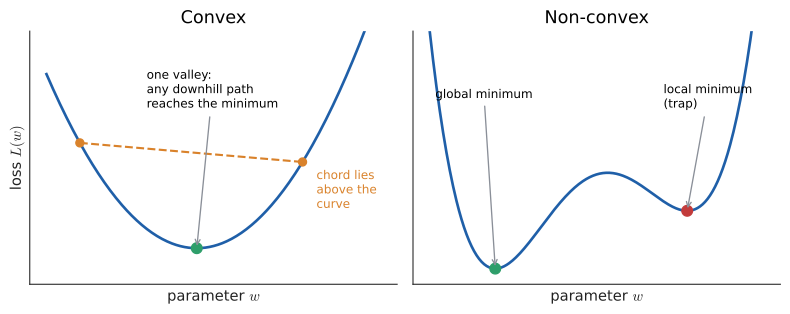
Linear regression (Section 33.2) and logistic regression (Section 33.3) have convex losses. Neural networks (Section 33.4) do not. One of the surprises of the last decade is that gradient descent still works astonishingly well on neural networks; why it works so well is an active research question.
33.1.4. The method: gradient descent and its variants
Recall the basic update from Chapter 20:
Here \(t\) counts steps, \(\eta\) (Greek eta) is the learning rate, and \(\nabla L(\theta_t)\) is the gradient of the loss at the current parameters. Two practical problems motivate two variants.
Problem 1: the gradient is expensive. In machine learning the loss is an average over a data set,
where \(\ell_i\) is the loss on example \(i\). If \(n\) is a billion, computing the exact gradient costs a billion evaluations per step. Stochastic gradient descent (SGD) instead estimates the gradient from a small random mini-batch of, say, 32 examples. The estimate is noisy but unbiased: on average it points the right way. You get a thousand cheap, slightly wobbly steps for the price of one exact step, and that is almost always a better deal.
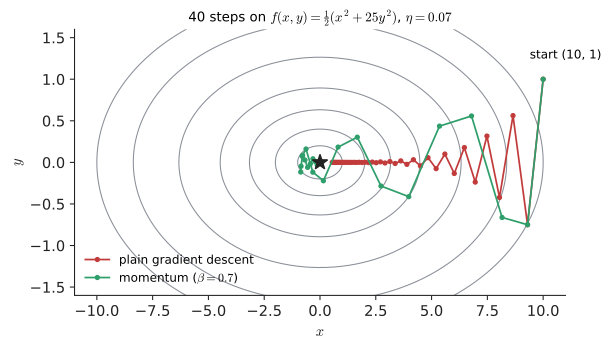
Problem 2: narrow valleys. If the landscape is a long, narrow ravine, the gradient points mostly across the ravine (where it is steep) rather than along it (where the minimum is). Plain gradient descent zig-zags from wall to wall and crawls along the floor. Momentum fixes this by letting the step accumulate a running "velocity": components of the gradient that keep pointing the same way (along the valley) build up, while components that flip sign every step (across the valley) cancel out.
|
Learning rate, mini-batch, epoch
The learning rate \(\eta\) is the step-size multiplier in gradient descent. A mini-batch is a small random subset of the training data used to estimate the gradient for one step. An epoch is one full pass through the training data — with 1,000 examples and batches of 32, one epoch is 32 steps (the last batch is short). Momentum \(\beta\) (Greek beta, typically 0.9) controls how much of the previous velocity carries into the next step. |
Input: a loss \(L(\theta) = \frac{1}{n}\sum_i \ell_i(\theta)\), a way to compute \(\nabla \ell_i\), initial parameters \(\theta_0\), learning rate \(\eta\), momentum \(\beta \in [0, 1)\), batch size \(B\), number of epochs.
Steps:
-
Set the velocity \(\mathbf{v} = \mathbf{0}\).
-
For each epoch: shuffle the example indices.
-
For each consecutive batch \(S\) of \(B\) indices:
-
Estimate the gradient: \(\mathbf{g} = \frac{1}{\lvert S\rvert}\sum_{i \in S} \nabla \ell_i(\theta)\).
-
Update the velocity: \(\mathbf{v} \leftarrow \beta \mathbf{v} + \mathbf{g}\).
-
Step: \(\theta \leftarrow \theta - \eta \mathbf{v}\).
-
-
Stop after the chosen number of epochs, or when the loss on held-out data stops improving.
Output: parameters \(\theta\) with (approximately) minimal loss.
With \(\beta = 0\) this is plain SGD; with \(\beta = 0\) and \(B = n\) it is plain (full-batch) gradient descent.
33.1.5. Worked example: momentum in a narrow valley
Take the ravine \(f(x, y) = \tfrac{1}{2}(x^2 + 25y^2)\). Its minimum is at the origin, but it is 25 times steeper in \(y\) than in \(x\). The gradient is Try it: Race momentum against descent.
Start at \((10, 1)\) with \(\eta = 0.07\).
Plain gradient descent, two steps.
The \(y\)-coordinate bounces \(1 \to -0.75 \to 0.5625\): it overshoots each time. The \(x\)-coordinate creeps down by only 7% per step.
Momentum with \(\beta = 0.7\), two steps. The first step is identical because the velocity starts at zero: \(\mathbf{v}_1 = (10, 25)\), position \((9.3, -0.75)\). Then
Look at what happened to the velocity. In \(x\), the old velocity and new gradient agreed, so the velocity grew to 16.3 and the step along the valley was 75% bigger. In \(y\), they disagreed (25 versus \(-18.75\)), so they almost cancelled and the bounce was damped. That is the whole idea of momentum, visible in two steps of arithmetic.
Now implement and run it for 100 steps:
import numpy as np

# A long, narrow valley: f(x, y) = 0.5*(x^2 + 25*y^2), minimum at (0, 0)
def grad(p):
    return np.array([p[0], 25.0 * p[1]])

def run(eta, beta, steps=100):
    p = np.array([10.0, 1.0])
    v = np.zeros(2)
    for _ in range(steps):
        v = beta * v + grad(p)          # velocity: running sum of gradients
        p = p - eta * v
    return np.linalg.norm(p)

print(f"plain GD  (beta=0.0): distance from minimum = {run(0.07, 0.0):.2e}")
print(f"momentum  (beta=0.7): distance from minimum = {run(0.07, 0.7):.2e}")
plain GD (beta=0.0): distance from minimum = 7.05e-03 momentum (beta=0.7): distance from minimum = 2.04e-07
You can predict the first number by hand: in \(x\) each plain step multiplies the coordinate by \(1 - 0.07 = 0.93\), and \(10 \times 0.93^{100} \approx 7.05 \times 10^{-3}\). Momentum is more than four orders of magnitude closer after the same number of gradient evaluations.
33.1.6. Alternative approaches and choosing a method
-
Closed form. Some problems (least squares, Section 33.2) can be solved exactly by setting the gradient to zero and solving the resulting equations. Use this when \(n\) and the number of parameters are moderate.
-
Newton’s method in several variables uses the Hessian as well as the gradient: \(\theta \leftarrow \theta - H^{-1}\nabla L\). It converges in very few steps near the minimum (quadratically, as in Chapter 32), but forming and inverting a \(p \times p\) Hessian costs \(O(p^3)\) — impossible for a network with \(p = 10^9\) parameters.
-
Adaptive methods such as Adam combine momentum with a per-parameter learning rate, scaled down for parameters whose gradients are consistently large. Adam is the default for training neural networks.
-
Derivative-free methods (grid search, random search, simulated annealing, evolutionary algorithms) need only function values. Use them when there is no gradient — for example tuning discrete hyperparameters.
A reasonable rule of thumb: closed form if it exists and fits in memory; Newton or quasi-Newton (L-BFGS) for smooth problems with up to a few thousand parameters; SGD with momentum or Adam for huge data and huge models; derivative-free when nothing else applies.
33.1.7. Constraints
Real problems have rules: probabilities must be non-negative and sum to 1, a robot arm’s joint angles are limited, a budget cannot be exceeded. A constrained problem is written
Three standard ways to handle the "subject to":
-
Lagrange multipliers (Chapter 20). At a constrained optimum on the boundary, the gradient of the objective is parallel to the gradient of the constraint: \(\nabla L = -\lambda \nabla g\). This turns a constrained problem into a system of equations, and generalises (as the Karush–Kuhn–Tucker conditions) to inequalities.
-
Projected gradient descent. Take an ordinary gradient step, then project back onto the allowed set — move to the nearest allowed point. For the constraint \(\theta \ge 0\) the projection is simply
max(theta, 0), applied component by component. -
Penalties. Replace the hard rule with a cost for breaking it: minimise \(L(\theta) + \lambda\, \lVert\theta\rVert^2\) instead of requiring \(\lVert\theta\rVert \le c\). This is exactly regularisation in machine learning (ridge regression, weight decay): it discourages large weights and reduces overfitting. The two forms are equivalent in the sense that every \(c\) corresponds to some \(\lambda\).
|
Learning rate is still the number-one failure
Every failure mode of gradient descent from Chapter 20 survives here. Too large a learning rate and the loss explodes, often to |
33.1.8. Where you’d use this
-
Packaging (everyday calculus). What shape of 330 ml drink can uses the least metal? With radius \(r\) and height \(h = 330/(\pi r^2)\), the surface area \(A(r) = 2\pi r^2 + 660/r\) is convex for \(r > 0\); setting \(A'(r) = 4\pi r - 660/r^2 = 0\) gives \(r = (330/2\pi)^{1/3} \approx 3.74\) cm and \(h = 2r \approx 7.5\) cm, area about 264 cm². Real cans are narrower (\(r \approx 3.3\) cm, so \(h \approx 9.6\) cm) and use only about 1.5% more metal: near a smooth minimum the loss is flat, so designers can trade a little optimality for a can that fits a hand and a vending machine. Try it: Design the drink can.
-
Physics: nature optimises. Light travels between two points along the path of least time (Fermat’s principle); minimising travel time across a boundary between air and water gives Snell’s law of refraction. A soap film minimises its area, and a hanging chain minimises its potential energy.
-
Engineering and logistics: aircraft wings are shaped by optimisers that minimise drag subject to lift and strength constraints; airlines schedule crews and delivery companies plan routes with linear and integer programming, constrained optimisation on a huge scale.
-
Finance: the minimum-variance portfolio of Chapter 30 is a constrained optimisation: minimise variance subject to the weights summing to 1.
|
Cauchy’s gradient descent
Gradient descent was proposed by Augustin-Louis Cauchy in 1847, in a three-page note on solving systems of equations arising from astronomical orbit calculations. Momentum is usually credited to Boris Polyak (1964), who called it the "heavy ball method" — the image is a ball rolling down the landscape, carrying its speed through small bumps. Stochastic approximation, the theory behind SGD, dates from Robbins and Monro in 1951. |
|
Optimiser race
Draw a 2-D loss landscape (a ravine, a bowl, an egg box). Drop a ball and choose plain gradient descent, momentum, or Adam, with sliders for \(\eta\) and \(\beta\). Watch the paths, count steps to reach the minimum, and find the learning rate where each method first diverges. On the egg box, try ten random starting points and see how many reach the global minimum. |
33.1.9. Exercises
-
Which of these are convex on all of \(\mathbb{R}\)? \(w^2\), \(\lvert w \rvert\), \(\sin w\), \(e^w\), \(w^3\).
-
Apply two steps of gradient descent to \(f(w) = (w - 3)^2\) from \(w_0 = 0\) with \(\eta = 0.1\). Then find a formula for \(w_t\), and the range of \(\eta\) for which the iteration converges.
-
Minimise \(f(w) = (w - 3)^2\) subject to \(w \le 2\) using projected gradient descent. What is the answer, and what does the projection do?
Answers
-
\(w^2\) (\(f'' = 2 \ge 0\)), \(\lvert w \rvert\) (chord check: the V-shape always lies below its chords), and \(e^w\) (\(f'' = e^w > 0\)) are convex. \(\sin w\) has \(f'' = -\sin w\), negative on \((0, \pi)\). \(w^3\) has \(f'' = 6w\), negative for \(w < 0\).
-
\(f'(w) = 2(w - 3)\). Step 1: \(w_1 = 0 - 0.1 \times 2(0 - 3) = 0 + 0.6 = 0.6\). Step 2: \(w_2 = 0.6 - 0.1 \times 2(0.6 - 3) = 0.6 + 0.48 = 1.08\). In general \(w_{t+1} - 3 = (w_t - 3) - 2\eta(w_t - 3) = (1 - 2\eta)(w_t - 3)\), so \(w_t = 3 + (1 - 2\eta)^t (w_0 - 3)\); with \(\eta = 0.1\), \(w_t = 3 - 3(0.8)^t\). It converges exactly when \(\lvert 1 - 2\eta \rvert < 1\), that is \(0 < \eta < 1\).
-
The unconstrained minimum \(w = 3\) is not allowed. Each gradient step pushes \(w\) towards 3; whenever it exceeds 2 the projection \(w \leftarrow \min(w, 2)\) clips it back. The iteration settles at \(w^* = 2\), on the boundary, with \(f(2) = 1\). At that point \(f'(2) = -2 \ne 0\): at a constrained optimum the gradient need not be zero, which is exactly what Lagrange multipliers account for.
33.2. Linear regression, end to end
33.2.1. The problem
You have recorded how many hours five students studied and their test scores (out of 6):
| hours \(x\) | 1 | 2 | 3 | 4 | 5 |
|---|---|---|---|---|---|
score \(y\) |
2 |
4 |
5 |
4 |
5 |
The points do not lie on a line, but there is clearly a trend. What is the best straight line through them? And what does "best" even mean?
This tiny question contains, in miniature, the whole workflow of machine learning: choose a model, choose a loss that says how wrong the model is, and optimise.
33.2.2. Intuition
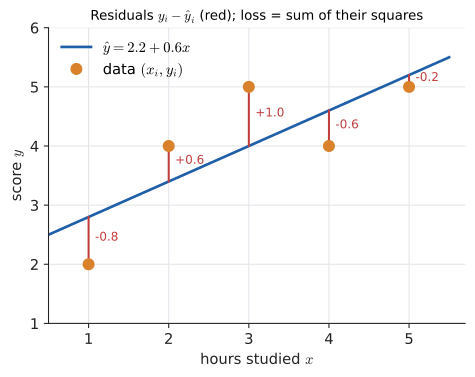
A line \(\hat y = b + wx\) makes a prediction \(\hat y_i\) (read "y-hat") for each \(x_i\). The vertical gap \(y_i - \hat y_i\) is the error, or residual. We want the residuals small, all at once. Adding them up fails — positive and negative errors cancel — so we square them first. Squaring makes every error count positively, punishes large errors more than small ones, and (crucially) produces a smooth, convex bowl that calculus can minimise exactly.
|
Residual, model, design matrix
A model is a function with adjustable parameters that maps inputs to predictions; here \(\hat y = b + wx\) with intercept \(b\) and slope (or weight) \(w\). A residual is \(r_i = y_i - \hat y_i\), observed minus predicted. The sum of squared errors is \(\text{SSE} = \sum_i r_i^2\); dividing by \(n\) gives the mean squared error (MSE). The design matrix \(X\) has one row per example and one column per parameter; for a line, row \(i\) is \(\lbrack 1,\ x_i]\), the 1 multiplying the intercept. |
33.2.3. Why it works: deriving the best line by calculus
The loss is a function of the two parameters:
At the minimum of a smooth bowl, both partial derivatives are zero (Chapter 20). Differentiate using the chain rule; the outer function is "square", the inner is \(y_i - b - wx_i\):
Set each to zero, divide by \(-2\), and split the sums:
These two linear equations in \(b\) and \(w\) are the normal equations. You know how to solve them from Chapter 6.
33.2.4. The method
Input: data points \((x_1, y_1), \dots, (x_n, y_n)\).
Steps:
-
Compute the four sums \(\sum x_i\), \(\sum y_i\), \(\sum x_i^2\), \(\sum x_i y_i\).
-
Write the normal equations \(\sum y_i = nb + w\sum x_i\) and \(\sum x_i y_i = b\sum x_i + w \sum x_i^2\).
-
Solve the 2-by-2 system for \(w\) and \(b\) (elimination, or the closed form \(w = \dfrac{\sum (x_i - \bar x)(y_i - \bar y)}{\sum (x_i - \bar x)^2}\), \(b = \bar y - w \bar x\)).
-
Optionally compute the residuals and the SSE to judge the fit.
Output: the line \(\hat y = b + wx\) minimising the sum of squared residuals.
33.2.5. Worked example
For the study data, \(n = 5\): Try it: Normal equations, step by step; Fit the least-squares line.
The normal equations are
Multiply the first by 3 and subtract it from the second:
So the best line is \(\hat y = 2.2 + 0.6x\): each extra hour of study is associated with 0.6 more points. The predictions at \(x = 1, \dots, 5\) are 2.8, 3.4, 4.0, 4.6, 5.2; the residuals are \(-0.8, 0.6, 1.0, -0.6, -0.2\) (they sum to zero, as the first normal equation guarantees); and
33.2.6. The same thing in matrix form
With many input features, writing out sums becomes hopeless. Matrices (Chapter 27) package it. Stack the parameters into \(\theta = [b,\ w]^{\mathsf T}\), the targets into \(\mathbf{y}\), and the inputs into the design matrix \(X\). Then all predictions at once are \(X\theta\), the residual vector is \(\mathbf{y} - X\theta\), and
That last line is the normal equations in matrix form, valid for any number of features. For the study data,
which are precisely the coefficients we found by hand. Two derivations, one by sums and partial derivatives, one by matrices and gradients, land on the same equations. That is a good sign you understand both.
|
Why "normal"?
The equations \(X^{\mathsf T}(\mathbf{y} - X\theta) = \mathbf{0}\) say that the residual vector is perpendicular ("normal", in the geometric sense) to every column of \(X\). Least squares is orthogonal projection: the best prediction \(X\theta\) is the shadow of \(\mathbf{y}\) on the space spanned by the columns of \(X\). Legendre published the method in 1805; Gauss claimed (credibly) to have used it since 1795, and famously used it to recover the lost dwarf planet Ceres from a handful of observations. |
33.2.7. Alternative approach: gradient descent
Instead of solving the equations, we can walk downhill on the MSE. Its gradient is \(\frac{2}{n}X^{\mathsf T}(X\theta - \mathbf{y})\). Starting from \(\theta = \mathbf{0}\) with \(\eta = 0.05\), the first step is Try it: Gradient descent versus the solve.
Both methods in code:
import numpy as np

# Data: hours studied (x) vs exam score (y)
x = np.array([1.0, 2.0, 3.0, 4.0, 5.0])
y = np.array([2.0, 4.0, 5.0, 4.0, 5.0])

# --- Method 1: closed form via the normal equations ---
X = np.column_stack([np.ones_like(x), x])    # design matrix: [1, x]
theta = np.linalg.solve(X.T @ X, X.T @ y)    # solve (X^T X) theta = X^T y
print("normal equations:", theta)

# --- Method 2: gradient descent on the mean squared error ---
def mse(theta):
    r = X @ theta - y
    return (r @ r) / len(y)

def grad(theta):
    return 2 * X.T @ (X @ theta - y) / len(y)

theta_gd = np.zeros(2)
eta = 0.05                                   # learning rate
for step in range(2001):
    theta_gd -= eta * grad(theta_gd)
    if step in (0, 10, 100, 1000, 2000):
        print(f"step {step:4d}  theta={theta_gd.round(4)}  loss={mse(theta_gd):.4f}")
normal equations: [2.2 0.6] step 0 theta=[0.4 1.32] loss=1.6464 step 10 theta=[0.6341 1.0337] loss=0.9263 step 100 theta=[1.8624 0.6935] loss=0.5007 step 1000 theta=[2.2 0.6] loss=0.4800 step 2000 theta=[2.2 0.6] loss=0.4800
Gradient descent takes about a thousand steps to match what the normal equations gave in one solve. On five points the closed form obviously wins. So why does anybody use gradient descent for regression?
And the stochastic version, on a thousand noisy points from the line \(y = 3x + 2\): Try it: Run SGD yourself.
import numpy as np

rng = np.random.default_rng(0)
n = 1000
x = rng.uniform(0, 10, n)
y = 3.0 * x + 2.0 + rng.normal(0, 1.0, n)     # true line: slope 3, intercept 2

w, b = 0.0, 0.0
eta, batch = 0.01, 32
for epoch in range(20):
    order = rng.permutation(n)                 # shuffle each epoch
    for start in range(0, n, batch):
        idx = order[start:start + batch]
        err = (w * x[idx] + b) - y[idx]
        w -= eta * 2 * np.mean(err * x[idx])   # gradient estimated from 32 points
        b -= eta * 2 * np.mean(err)
print(f"SGD estimate: slope {w:.2f}, intercept {b:.2f}")
X = np.column_stack([np.ones(n), x])
b_exact, w_exact = np.linalg.solve(X.T @ X, X.T @ y)
print(f"Exact least squares: slope {w_exact:.2f}, intercept {b_exact:.2f}")
SGD estimate: slope 3.11, intercept 1.93 Exact least squares: slope 3.00, intercept 2.00
SGD lands close but not exactly on the answer: with a constant learning rate it keeps jittering around the minimum, as the Watch out box in Section 33.1 warned. Decaying \(\eta\) over the epochs would tighten it.
33.2.8. Choosing a method
-
Normal equations (
np.linalg.solve(X.T @ X, X.T @ y)): fine when the number of features \(p\) is up to a few thousand. Cost \(O(np^2 + p^3)\). -
QR decomposition or
np.linalg.lstsq: the numerically preferred closed form. Forming \(X^{\mathsf T}X\) squares the condition number (Chapter 32), so nearly collinear features lose twice as many digits; QR works on \(X\) directly. This is what statistical software actually does. -
Gradient descent / SGD: when \(n\) is too large to fit in memory, when data arrive as a stream, or when the model is not linear (then there is no closed form at all, and gradient descent is the only game in town). Learning it on a problem where you can check the answer is the point of this section.
|
Least squares has blind spots
|
Try it: Outliers: squared versus absolute.
33.2.9. Where you’d use this
-
Astronomy: the age of the universe. Plot the recession speeds of galaxies against their distances and fit a line through the origin: the slope is the Hubble constant, about 70 km/s per megaparsec. Its reciprocal, converted to years, is about 14 billion years, a first estimate of the age of the universe from a least-squares slope.
-
Everyday: pricing. Regress house prices on floor area in your town and the slope is the price per extra square metre; estate agents' "comparable sales" valuations are an informal version, and automated valuation websites use multiple regression with dozens of features.
-
Science and medicine: dose against response, temperature against reaction rate (after taking logarithms, as in the Arrhenius equation), and height against age on a growth chart are all fitted by least squares; the fitted coefficients are the scientific result.
|
Drag the points
Plot five to twenty points and the least-squares line. Drag any point and watch the line, the residual squares, and the SSE update live. Drag one point far away to feel how an outlier pulls the line. Toggle between squared and absolute error and compare. |
33.2.10. Exercises
-
Fit the least-squares line to \((0, 1), (1, 3), (2, 5)\). What is the SSE?
-
Fit the least-squares line to \((1, 1), (2, 2), (3, 2), (4, 4)\), showing the four sums.
-
For a line through the origin, \(\hat y = wx\), derive the least-squares slope.
Answers
-
The points lie exactly on \(y = 2x + 1\), so that line has every residual zero and SSE \(= 0\); no line can do better. (Check with sums: \(n = 3\), \(\sum x = 3\), \(\sum y = 9\), \(\sum x^2 = 5\), \(\sum xy = 13\); equations \(9 = 3b + 3w\), \(13 = 3b + 5w\); subtracting gives \(4 = 2w\), so \(w = 2\), \(b = 1\).)
-
\(n = 4\), \(\sum x = 10\), \(\sum y = 9\), \(\sum x^2 = 30\), \(\sum xy = 1 + 4 + 6 + 16 = 27\). Equations: \(9 = 4b + 10w\) and \(27 = 10b + 30w\). Multiply the first by 2.5: \(22.5 = 10b + 25w\). Subtract: \(4.5 = 5w\), so \(w = 0.9\), and \(4b = 9 - 9 = 0\), so \(b = 0\). Line: \(\hat y = 0.9x\).
-
\(L(w) = \sum (y_i - wx_i)^2\), \(L'(w) = -2\sum x_i(y_i - wx_i) = 0 \Rightarrow \sum x_i y_i = w \sum x_i^2 \Rightarrow w = \sum x_i y_i / \sum x_i^2\). Since \(L''(w) = 2\sum x_i^2 > 0\), this is a minimum.
33.3. Logistic regression: from lines to probabilities
33.3.1. The problem
Now the question is yes/no. Ten students studied for between half an hour and five hours; some passed (1) and some failed (0):
| hours | 0.5 | 1.0 | 1.5 | 2.0 | 2.5 | 3.0 | 3.5 | 4.0 | 4.5 | 5.0 |
|---|---|---|---|---|---|---|---|---|---|---|
passed |
0 |
0 |
0 |
1 |
0 |
1 |
0 |
1 |
1 |
1 |
We want a model that outputs the probability of passing. A straight line is wrong for the job: it happily predicts probabilities of \(-0.3\) or 1.4, and a single extreme student drags it around. We need a function that takes any real number and squeezes it into \((0, 1)\).
33.3.2. Intuition: the sigmoid
The sigmoid (or logistic) function is
Read it piece by piece. For large positive \(z\), \(e^{-z}\) is tiny, so \(\sigma(z) \approx 1/1 = 1\). For large negative \(z\), \(e^{-z}\) is huge, so \(\sigma(z) \approx 0\). At \(z = 0\), \(\sigma(0) = 1/(1+1) = 1/2\). It is an S-shaped curve that turns a "score" of any size into a probability.
Logistic regression computes a linear score and passes it through the sigmoid:
|
Odds, logit, sigmoid
The odds of an event with probability \(p\) are \(p/(1-p)\): a probability of 0.8 is odds of 4 to 1. The logit is the log-odds, \(\operatorname{logit}(p) = \ln\frac{p}{1-p}\), which runs over all of \(\mathbb{R}\). The sigmoid \(\sigma(z) = 1/(1 + e^{-z})\) is the inverse of the logit. So logistic regression says: the log-odds are a linear function of the input. Each extra unit of \(x\) multiplies the odds by \(e^{w}\). |
33.3.3. Why it works: the loss comes from probability
What should the loss be? Squared error is tempting but leads to a non-convex problem here. A principled answer comes from probability (Chapter 29): choose \(w, b\) to make the observed data as likely as possible — maximum likelihood.
If the model says student \(i\) passes with probability \(p_i\), then the probability of the observed outcome \(y_i \in \{0, 1\}\) is \(p_i\) if they passed and \(1 - p_i\) if they failed. A neat way to write both cases at once is \(p_i^{y_i}(1-p_i)^{1-y_i}\) (one of the exponents is always zero). Treating students as independent, the likelihood of the whole data set is the product, and
The symbol \(\prod\) (capital Greek pi) is the product analogue of \(\sum\): multiply the terms rather than add them. The final expression is the binary cross-entropy loss. You will see in Section 33.6 that "cross-entropy" is a precise term from information theory, not a coincidence of naming.
|
Cross-entropy loss
For a true label \(y \in \{0, 1\}\) and predicted probability \(p\), the binary cross-entropy is \(-[y\ln p + (1-y)\ln(1-p)]\). If \(y = 1\) it is \(-\ln p\): zero when \(p = 1\), growing without bound as \(p \to 0\). Confident wrong answers are punished severely. It is also called log loss or negative log-likelihood. |
33.3.4. Deriving the gradient
The gradient turns out to be beautifully simple. Two ingredients.
Derivative of the sigmoid. Write \(\sigma(z) = (1 + e^{-z})^{-1}\) and use the chain rule:
Derivative of the loss for one example. Let \(\ell = -[y\ln p + (1-y)\ln(1-p)]\) with \(p = \sigma(z)\), \(z = wx + b\). Chain rule, link by link:
The gradient is "prediction minus truth, times input" — exactly the same shape as for linear regression. The messy sigmoid derivative cancelled perfectly against the logarithms. That cancellation is no accident; it is why cross-entropy and sigmoid are always used together.
33.3.5. The method and a worked run
Input: examples \((x_i, y_i)\) with \(y_i \in \{0, 1\}\); learning rate \(\eta\); number of steps.
Steps:
-
Initialise \(w = 0\), \(b = 0\).
-
Repeat:
-
Compute predictions \(p_i = \sigma(wx_i + b)\) for all \(i\).
-
Compute gradients \(g_w = \frac{1}{n}\sum (p_i - y_i)x_i\) and \(g_b = \frac{1}{n}\sum(p_i - y_i)\).
-
Update \(w \leftarrow w - \eta g_w\), \(b \leftarrow b - \eta g_b\).
-
-
Stop when the gradients are near zero or the loss stops improving.
Output: \(w, b\); predict \(P(y = 1 \mid x) = \sigma(wx + b)\), and classify as 1 when this exceeds a threshold (often 0.5).
Try it: The fitted logistic curve.
By hand, the first step: with \(w = b = 0\) every \(p_i = \sigma(0) = 0.5\). Five students passed and five failed, so
and \(b\) does not move yet. For \(w\) we need \(\sum_i x_i = 27.5\) and the sum of the passers' hours, \(2.0 + 3.0 + 4.0 + 4.5 + 5.0 = 18.5\):
The slope starts positive: more hours, higher pass probability. The code runs the same update 5,000 times.
import numpy as np

def sigmoid(z):
    return 1.0 / (1.0 + np.exp(-z))

# Hours studied -> passed (1) or failed (0)
x = np.array([0.5, 1.0, 1.5, 2.0, 2.5, 3.0, 3.5, 4.0, 4.5, 5.0])
y = np.array([0,   0,   0,   1,   0,   1,   0,   1,   1,   1  ])

w, b = 0.0, 0.0
eta = 0.1
for step in range(5000):
    p = sigmoid(w * x + b)                 # predicted probabilities
    w -= eta * np.mean((p - y) * x)        # dL/dw
    b -= eta * np.mean(p - y)              # dL/db

p = sigmoid(w * x + b)
loss = -np.mean(y * np.log(p) + (1 - y) * np.log(1 - p))
print(f"w={w:.3f}  b={b:.3f}  cross-entropy={loss:.3f}")
print(f"P(pass | 1 hour)  = {sigmoid(w*1 + b):.3f}")
print(f"P(pass | 4 hours) = {sigmoid(w*4 + b):.3f}")
print(f"50% boundary at x = {-b/w:.2f} hours")
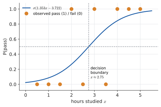
w=1.353 b=-3.721 cross-entropy=0.434 P(pass | 1 hour) = 0.086 P(pass | 4 hours) = 0.844 50% boundary at x = 2.75 hours
Check one prediction by hand: at one hour, \(z = 1.353 - 3.721 = -2.368\), \(e^{2.368} \approx 10.68\), and \(\sigma(-2.368) = 1/(1 + 10.68) \approx 0.086\). The decision boundary is where \(p = 0.5\), that is where \(z = 0\): \(x = -b/w = 3.721/1.353 \approx 2.75\) hours. The slope means each extra hour multiplies the odds of passing by \(e^{1.353} \approx 3.9\).
33.3.6. Alternatives and choosing
Logistic regression is the natural first model for binary classification: convex (so training always finds the best fit), fast, and interpretable — each weight is a log-odds ratio you can explain to a colleague. Alternatives include decision trees and gradient-boosted trees (often more accurate on tabular data, less interpretable), support-vector machines, and neural networks, which are, as the next section shows, stacked logistic regressions. With more than two classes, the sigmoid generalises to the softmax (Section 33.9).
|
Perfect separation and log(0)
|
33.3.7. Where you’d use this
-
Medicine: risk calculators. Clinical risk scores that estimate, say, the 10-year probability of a heart attack from age, blood pressure, cholesterol and smoking are logistic (or closely related) regressions fitted to large patient studies. Each weight has a direct reading: a weight of 0.7 on "smoker" multiplies the odds by \(e^{0.7} \approx 2\).
-
Pharmacology: dose–response. The fraction of patients who respond to a dose follows an S-curve in log-dose; the dose where the curve crosses 50% (the decision boundary \(x = -b/w\)) is the drug’s ED50, the number on which dosing is based.
-
Finance: credit scoring turns an applicant’s history into a probability of default with a logistic model, and regulators like it precisely because each weight can be explained to a rejected customer.
|
Logistic curve explorer
Plot pass/fail data and a sigmoid with sliders for \(w\) and \(b\). Show the cross-entropy loss live, and a second panel with the loss surface over \((w, b)\) as a contour plot with a dot for the current setting. Then press "train" and watch gradient descent slide the dot to the bottom of the (convex) bowl. |
33.3.8. Exercises
-
Compute \(\sigma(0)\), \(\sigma(2)\), \(\sigma(-2)\). What do you notice about the last two?
-
A model predicts \(p = 0.9\) for an example whose true label is 1. What is the cross-entropy loss? What if it predicts \(p = 0.1\)?
-
Show algebraically that \(\sigma(-z) = 1 - \sigma(z)\).
Answers
-
\(\sigma(0) = 0.5\); \(\sigma(2) = 1/(1 + e^{-2}) = 1/1.1353 \approx 0.881\); \(\sigma(-2) = 1/(1 + e^{2}) = 1/8.389 \approx 0.119\). They sum to 1 — see exercise 3.
-
\(-\ln 0.9 \approx 0.105\); \(-\ln 0.1 \approx 2.303\). Being confidently wrong costs about 22 times as much as being fairly confidently right.
-
\(\sigma(-z) = \dfrac{1}{1 + e^{z}} = \dfrac{e^{-z}}{e^{-z} + 1}\) (multiply top and bottom by \(e^{-z}\)) \(= \dfrac{(1 + e^{-z}) - 1}{1 + e^{-z}} = 1 - \dfrac{1}{1 + e^{-z}} = 1 - \sigma(z)\).
33.4. Neurons, networks, and the chain rule
33.4.1. The problem
Logistic regression draws a single straight boundary. Many real problems need curved, tangled boundaries: recognising a handwritten 7, deciding whether a sentence is sarcastic. We want a model flexible enough to learn any reasonable function from data, yet still trainable by gradient descent.
33.4.2. Intuition: functions composed with functions
An artificial neuron is exactly logistic regression with several inputs:
It takes a weighted sum of its inputs (a dot product, Chapter 26), adds a bias, and applies a nonlinear activation function. A layer is many neurons side by side, which in matrix form is \(\mathbf{a} = \sigma(W\mathbf{x} + \mathbf{b})\) with \(\sigma\) applied to each component. A network is layers stacked, each feeding the next:
That is all a neural network is: a composition of simple functions (Chapter 11), with a very large number of adjustable parameters.
|
Neuron, activation, layer
A neuron computes \(\phi(\mathbf{w}\cdot\mathbf{x} + b)\) for weights \(\mathbf{w}\), bias \(b\), and activation function \(\phi\) (Greek phi). Common activations: the sigmoid \(\sigma\); \(\tanh\); and the ReLU (rectified linear unit) \(\operatorname{ReLU}(z) = \max(0, z)\). A layer applies many neurons to the same input. A hidden layer is any layer between input and output. The forward pass evaluates the network; the backward pass computes gradients. |
33.4.3. Why the nonlinearity matters
Why not drop the activation and just stack linear layers? Because the composition of linear maps is linear: Try it: Train without an activation.
A hundred linear layers collapse into one matrix (Chapter 27), so the "deep" network would be no more expressive than linear regression. The nonlinearity between layers is what lets each layer bend the space the next one sees. The universal approximation theorem makes this precise: one hidden layer with enough sigmoid (or ReLU) neurons can approximate any continuous function on a bounded region as closely as you like.
33.4.4. Why training works: backpropagation is the chain rule
To train with gradient descent, we need \(\partial L / \partial w\) for every weight. The loss is a long composition, and the chain rule (Chapter 17, and its multivariable form in Chapter 20) says: the derivative of a composition is the product of the derivatives of the links. Backpropagation is nothing more than evaluating that product efficiently, starting from the loss and working backwards, reusing each intermediate result.
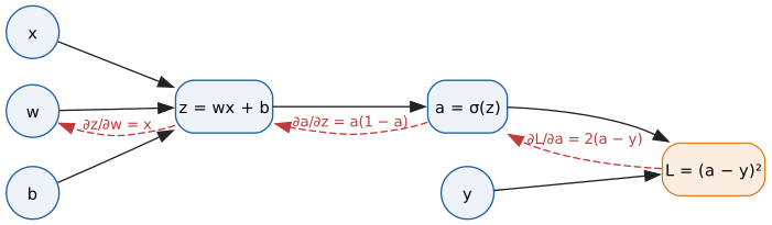
Input: a computation expressed as a sequence of steps \(u_1 \to u_2 \to \dots \to L\), each with a known local derivative; parameter values.
Steps:
-
Forward pass: compute and store every intermediate value \(u_1, u_2, \dots, L\).
-
Set \(\partial L / \partial L = 1\).
-
Backward pass: for each step in reverse order, multiply the incoming gradient by that step’s local derivative: \(\dfrac{\partial L}{\partial u_k} = \dfrac{\partial L}{\partial u_{k+1}}\cdot\dfrac{\partial u_{k+1}}{\partial u_k}\). Where a value feeds several later steps, add the contributions.
-
Read off \(\partial L/\partial(\text{parameter})\) for each parameter.
Output: the gradient of the loss with respect to every parameter, at a cost of roughly two forward passes.
33.4.5. Worked example
One neuron, squared-error loss: input \(x = 2\), target \(y = 1\), weight \(w = 0.5\), bias \(b = -1\). Try it: Backprop through one neuron.
Forward pass.
Backward pass, outermost link first:
Both gradients are negative, so gradient descent will increase \(w\) and \(b\), pushing \(a\) up towards the target 1. Now verify against a finite difference (Chapter 32) — the standard "gradient check" every ML engineer learns to do:
import numpy as np

# One neuron: y_hat = sigmoid(w*x + b), squared-error loss
x, y = 2.0, 1.0
w, b = 0.5, -1.0

z = w * x + b                    # forward pass, step 1
a = 1 / (1 + np.exp(-z))         # forward pass, step 2
L = (a - y) ** 2                 # forward pass, step 3

dL_da = 2 * (a - y)              # backward pass: outermost link first
da_dz = a * (1 - a)
dz_dw = x
dL_dw = dL_da * da_dz * dz_dw    # chain rule: multiply the links
dL_db = dL_da * da_dz * 1.0

print(f"z={z:.4f} a={a:.4f} L={L:.4f}")
print(f"dL/dw={dL_dw:.4f}  dL/db={dL_db:.4f}")

# Check against a finite difference
h = 1e-6
L2 = (1 / (1 + np.exp(-((w + h) * x + b))) - y) ** 2
print(f"finite-difference dL/dw = {(L2 - L) / h:.4f}")
z=0.0000 a=0.5000 L=0.2500 dL/dw=-0.5000 dL/db=-0.2500 finite-difference dL/dw = -0.5000
In a real network the same pattern repeats through every layer. The vector form of each link is a Jacobian matrix (Chapter 20), and the backward pass is a chain of matrix–vector products, which is why GPUs — machines built for matrix multiplication — train networks so well.
33.4.6. Why backward and not forward?
You could apply the chain rule from the inputs forwards instead. For a function with one input and many outputs that would be efficient. But a loss has one output and millions of inputs (the parameters). Going backwards, one pass gives the derivative with respect to all of them at once; going forwards would need one pass per parameter. This is reverse-mode automatic differentiation, and the asymmetry is the entire reason deep learning is computationally feasible.
|
Vanishing gradients
The sigmoid’s derivative \(\sigma(1-\sigma)\) is at most \(1/4\) (at \(z = 0\)) and nearly zero when the neuron is saturated near 0 or 1. Backpropagation multiplies one such factor per layer, so through 20 sigmoid layers the gradient can shrink by a factor of \((1/4)^{20} \approx 10^{-12}\) — early layers stop learning. This vanishing gradient problem is why modern networks use ReLU (derivative exactly 1 for positive inputs), careful initialisation, and "residual connections" that give gradients a shortcut. The opposite, exploding gradients, happens when the factors exceed 1; the fix is gradient clipping. |
33.4.7. Where you’d use this
-
Everyday: face unlock on a phone, speech-to-text, photo search ("show me pictures of dogs"), live translation and the predictive keyboard are all neural networks trained by backpropagation.
-
Science and medicine: AlphaFold predicts the 3-D shape of proteins from their amino-acid sequence (its designers shared the 2024 Nobel Prize in Chemistry); networks screen retinal photographs for diabetic eye disease; weather services now run neural forecasting models alongside the physics-based ones.
-
Engineering: a network trained on thousands of slow physics simulations can act as a fast surrogate model, letting engineers explore millions of designs in the time one full simulation used to take.
|
Backpropagation’s many inventors
Reverse-mode automatic differentiation was described by Seppo Linnainmaa in his 1970 master’s thesis; Paul Werbos applied it to neural networks in 1974; and the 1986 Nature paper by Rumelhart, Hinton and Williams made it famous. The perceptron — a single neuron with a step activation — dates from Frank Rosenblatt in 1958, and the idea of a neuron as a weighted threshold unit from McCulloch and Pitts in 1943. |
|
Neuron playground
Build a tiny network (2 inputs, one hidden layer of up to 8 neurons, 1 output) and train it on a 2-D data set: two blobs, a circle inside a ring, a spiral. Watch the decision boundary bend as training proceeds. Remove the activation function and confirm that the boundary stays a straight line no matter how many layers you add. Hover over any weight to see its current gradient. Try it: Train a tiny network |
33.4.8. Exercises
-
Explain in one sentence why a network with no activation functions cannot learn the boundary "inside versus outside a circle". Try it: Check the exercise.
-
Repeat the worked example with \(x = 1\), \(y = 0\), \(w = 1\), \(b = 0\). Find \(L\) and \(\partial L/\partial w\).
-
What is the derivative of \(\operatorname{ReLU}(z)\)? Why is it less prone to vanishing gradients?
Answers
-
Without activations the whole network is a single linear map, whose decision boundary \(\mathbf{w}\cdot\mathbf{x} + b = 0\) is a straight line (a hyperplane), and no straight line separates the inside of a circle from the outside.
-
\(z = 1\), \(a = \sigma(1) \approx 0.7311\), \(L = 0.7311^2 \approx 0.5344\). \(\partial L/\partial a = 2(0.7311 - 0) \approx 1.4621\); \(\partial a/\partial z = 0.7311 \times 0.2689 \approx 0.1966\); \(\partial z/\partial w = x = 1\). So \(\partial L/\partial w \approx 1.4621 \times 0.1966 \approx 0.2875\): positive, so gradient descent decreases \(w\), lowering \(a\) towards 0.
-
It is 0 for \(z < 0\) and 1 for \(z > 0\) (undefined at 0; libraries pick 0). For active neurons the local factor is exactly 1, so it does not shrink the gradient layer after layer the way \(\sigma' \le 1/4\) does.
33.5. Embeddings, dot products, and search
33.5.1. The problem
You type "cat on mat" into a search box. Out of millions of documents, which should come first? Computers cannot compare meanings directly; they compare numbers. So the plan is: turn every document and every query into a vector, and measure how well they match with a single arithmetic operation. That operation is the dot product, and this is the \(\mathbf{q}\cdot\mathbf{d}\) you will meet in every information-retrieval paper.
33.5.2. Intuition
Give every possible word its own axis. A document becomes a point (a vector) in this enormous space, with coordinate \(j\) saying how important word \(j\) is to the document. Documents about similar things point in similar directions. The query is a vector too. "How relevant is document \(\mathbf{d}\) to query \(\mathbf{q}\)?" becomes "how closely do the two arrows point the same way?"
Recall from Chapter 26 that
so the dot product mixes two things: the angle between the vectors (what we care about — topic) and their lengths (often an accident of document length). Dividing the lengths out gives cosine similarity:
It is 1 for vectors pointing the same way, 0 for perpendicular (no shared words), and \(-1\) for opposite directions (impossible for word counts, which are non-negative, but common for learned embeddings).
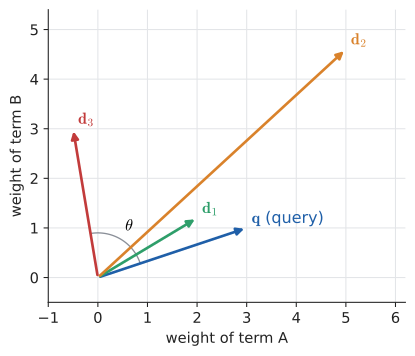
|
Cosine similarity, norm, unit vector
The norm (length) of a vector is \(\lVert\mathbf{v}\rVert = \sqrt{\mathbf{v}\cdot\mathbf{v}} = \sqrt{\sum_j v_j^2}\). A unit vector has norm 1; normalising means dividing by the norm. Cosine similarity is the dot product of the two normalised vectors. For unit vectors, dot product and cosine similarity are the same number — which is why systems often normalise everything once at indexing time and then just take dot products. |
33.5.3. Turning text into vectors: TF-IDF
Raw counts give too much weight to words like "the". Two adjustments fix this:
-
Term frequency \(\operatorname{tf}(t, d)\): how often term \(t\) appears in document \(d\). More mentions, more relevant.
-
Inverse document frequency \(\operatorname{idf}(t) = \ln\dfrac{N}{\operatorname{df}(t)}\), where \(N\) is the number of documents and \(\operatorname{df}(t)\) the number containing \(t\). A word in every document gets \(\ln 1 = 0\): it tells you nothing. A rare word gets a large weight.
The weight of term \(t\) in document \(d\) is \(\operatorname{tf}(t,d)\times\operatorname{idf}(t)\). The logarithm (Chapter 12) is there to compress the scale: a word in 1 document out of a million should count for more than one in 1,000, but not a thousand times more.
33.5.4. Worked example
Three documents and a query: Try it: TF-IDF for “cat on mat”.
-
d1: "the cat sat on the mat"
-
d2: "the dog sat on the log"
-
d3: "cats and dogs are pets"
-
query: "cat on mat"
With \(N = 3\): "cat" and "mat" appear only in d1, so \(\operatorname{idf} = \ln 3 \approx 1.0986\). "on", "the" and "sat" appear in two documents: \(\operatorname{idf} = \ln(3/2) \approx 0.4055\). The query vector has non-zero entries only for cat, on and mat, so only those coordinates of each document matter for the dot product:
d1 wins decisively. Note that "the" (twice in d1) contributes nothing to the dot product because the query does not contain it — but it does lengthen \(\mathbf{d}_1\), which the cosine will account for. The code computes both scores:
import math
from collections import Counter

docs = {
    "d1": "the cat sat on the mat",
    "d2": "the dog sat on the log",
    "d3": "cats and dogs are pets",
}
query = "cat on mat"

tokenised = {name: text.split() for name, text in docs.items()}
vocab = sorted({w for words in tokenised.values() for w in words})
N = len(docs)
df = {w: sum(w in words for words in tokenised.values()) for w in vocab}
idf = {w: math.log(N / df[w]) for w in vocab}

def tfidf(words):
    counts = Counter(words)
    return [counts[w] * idf.get(w, 0.0) for w in vocab]

def dot(u, v):
    return sum(a * b for a, b in zip(u, v))

def cosine(u, v):
    nu, nv = math.sqrt(dot(u, u)), math.sqrt(dot(v, v))
    return dot(u, v) / (nu * nv) if nu and nv else 0.0

q = tfidf(query.split())
for name, words in tokenised.items():
    d = tfidf(words)
    print(f"{name}: q.d = {dot(q, d):.3f}   cos = {cosine(q, d):.3f}")
d1: q.d = 2.578 cos = 0.871 d2: q.d = 0.164 cos = 0.056 d3: q.d = 0.000 cos = 0.000
33.5.5. Alternatives: BM25 and learned embeddings
BM25, the default ranking function in search engines such as Lucene, Elasticsearch and OpenSearch, refines TF-IDF in two ways. Its score is Try it: Tune BM25’s k₁ and b.
Read it piece by piece: for each query term, an IDF weight times a saturating function of the term count \(f(t,d)\). The fraction approaches \(k_1 + 1\) as the count grows, so the tenth mention of "cat" adds much less than the first. The bracket in the denominator normalises for document length \(\lvert d\rvert\) relative to the average length "avgdl": \(b = 0\) ignores length, \(b = 1\) normalises fully. Typical settings are \(k_1 \approx 1.2\) and \(b = 0.75\).
Dense embeddings replace the hand-built word axes with a few hundred learned dimensions. A neural network (Section 33.4) is trained so that texts with similar meanings get vectors with high cosine similarity — so "feline resting on a rug" lands near "cat on mat" despite sharing no words. The retrieval step is unchanged: \(\mathbf{q}\cdot\mathbf{d}\), usually on unit vectors.
|
Embedding
An embedding is a map from discrete objects (words, sentences, images, users, products) to vectors in \(\mathbb{R}^k\), chosen so that geometric relationships reflect real ones: similar objects get nearby vectors. Sparse embeddings (TF-IDF) have one dimension per vocabulary word and mostly zeros; dense embeddings have a few hundred learned dimensions, all typically non-zero. |
Choosing. BM25 is fast, needs no training, and is excellent for exact keyword matches (error codes, names, part numbers). Dense embeddings capture meaning and synonyms but can miss rare exact terms and need a model. Modern systems often run both and combine the scores ("hybrid search").
|
Tokenisation and length traps
|
33.5.6. Where you’d use this
-
Everyday: recommendations. A music service represents each listener and each song as a vector; songs whose vectors have a high cosine with yours are recommended, and "people who liked this also liked" compares item vectors with each other. The same geometry powers "similar products" in online shops and "more like this" on video sites.
-
Chemistry and drug discovery: a molecule is encoded as a long 0/1 vector ("fingerprint") recording which structural fragments it contains; chemists search libraries of millions of compounds for molecules similar to a promising drug using a cosine-like overlap score (the Tanimoto coefficient).
-
Biology: DNA and protein sequences are compared by counting shared short substrings, a TF-IDF-like vector that lets search tools find related genes in seconds.
|
king − man + woman ≈ queen
In the word2vec embeddings published by Mikolov and colleagues in 2013, vector arithmetic captured analogies: the vector \(\mathbf{v}_{\text{king}} - \mathbf{v}_{\text{man}} + \mathbf{v}_{\text{woman}}\) was closer to \(\mathbf{v}_{\text{queen}}\) than to any other word. Directions in the space had come to mean things ("royalty", "gender") without anyone telling the model. TF-IDF is much older: Karen Spärck Jones introduced inverse document frequency in 1972. |
|
Search engine in a box
Type a handful of short documents and a query. See the vocabulary, the TF-IDF vectors as a table, the dot product and cosine for each document, and the ranking. Toggle stemming on and off; switch between TF-IDF and BM25 and move the \(k_1\) and \(b\) sliders to see how term saturation and length normalisation reorder the results. Try it: Search engine in a box |
33.5.7. Exercises
-
Compute the cosine similarity of \((1, 0)\) and \((0, 1)\), and of \((1, 2)\) and \((2, 4)\).
-
For \(\mathbf{q} = (1, 1, 0)\), \(\mathbf{d}_1 = (2, 2, 0)\), \(\mathbf{d}_2 = (1, 0, 1)\), compute both dot products and both cosines. Which document wins under each?
-
In the worked example, why does adding the word "the" ten more times to d1 leave \(\mathbf{q}\cdot\mathbf{d}_1\) unchanged but lower its cosine?
Answers
-
\((1,0)\cdot(0,1) = 0\), so cosine 0 (perpendicular). \((1,2)\cdot(2,4) = 2 + 8 = 10\); norms \(\sqrt 5\) and \(\sqrt{20}\), product \(\sqrt{100} = 10\); cosine 1 (same direction, different length).
-
\(\mathbf{q}\cdot\mathbf{d}_1 = 2 + 2 + 0 = 4\), \(\mathbf{q}\cdot\mathbf{d}_2 = 1 + 0 + 0 = 1\). Cosines: \(4/(\sqrt2\cdot\sqrt8) = 4/4 = 1\) and \(1/(\sqrt2\cdot\sqrt2) = 0.5\). \(\mathbf{d}_1\) wins under both.
-
The query has weight 0 on "the", so that coordinate contributes \(0 \times (\text{anything}) = 0\) to the dot product. But the extra occurrences increase \(\lVert\mathbf{d}_1\rVert\), the denominator of the cosine, so the cosine falls.
33.6. Information theory: measuring surprise
33.6.1. The problem
How much information is in a message? A file compressor has to answer this concretely: how few bits can it get away with? A language model is graded by how well it predicts the next word — but what number measures "well"? And the logistic-regression loss was called cross-entropy. Why?
All three questions have one answer, due to Claude Shannon in 1948.
33.6.2. Intuition: information is surprise
Learning that something likely happened tells you little; learning that something unlikely happened tells you a lot. "The sun rose this morning" carries almost no information. "It snowed in July in Miami" carries a great deal.
Think of the game of twenty questions. If a number is chosen uniformly from 1 to 8, you can always find it with three yes/no questions ("Is it in the top half?"), because each answer halves the possibilities: \(8 \to 4 \to 2 \to 1\). An event of probability \(1/8\) needs 3 bits to pin down; \(3 = \log_2 8 = -\log_2(1/8)\).
That suggests defining the surprise (or self-information) of an event with probability \(p\) as
Certain events (\(p = 1\)) have surprise 0. Each halving of probability adds one bit. And because logs turn products into sums (Chapter 12), the surprise of two independent events is the sum of their surprises — exactly what "amount of information" ought to do.
33.6.3. Entropy: average surprise
A random source — a coin, a die, the next letter of English text — produces outcomes with probabilities \(p_1, \dots, p_k\). Its entropy is the expected surprise (expectation from Chapter 29):
(By convention \(0\log 0 = 0\): impossible outcomes contribute nothing.)
|
Bit, surprise, entropy
A bit is the information in one fair yes/no answer. The surprise or self-information of an outcome with probability \(p\) is \(-\log_2 p\) bits. Entropy \(H\) is average surprise: the uncertainty of a random source before you see the outcome. With natural logarithms the unit is the nat (\(1 \text{ nat} \approx 1.443\) bits); ML papers often use nats without saying so. |
33.6.4. Worked examples
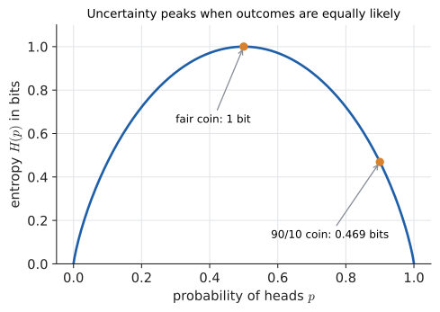
Fair coin. \(H = -\big(\tfrac12\log_2\tfrac12 + \tfrac12\log_2\tfrac12\big) = -\big(\tfrac12(-1) + \tfrac12(-1)\big) = 1\) bit. Try it: Entropy and its Huffman code.
Biased coin with \(P(\text{heads}) = 0.9\):
The biased coin is more predictable, so it carries less than half a bit per flip.
Fair die. Six outcomes of probability \(1/6\): \(H = -6 \times \tfrac16\log_2\tfrac16 = \log_2 6 \approx 2.585\) bits. In general a uniform distribution over \(k\) outcomes has entropy \(\log_2 k\), the maximum possible for \(k\) outcomes.
A skewed four-symbol source with probabilities \(\tfrac12, \tfrac14, \tfrac18, \tfrac18\):
33.6.5. Why compression connects to probability
Here is the payoff. For the four-symbol source, use the code
| symbol | probability | codeword | length |
|---|---|---|---|
A |
1/2 |
|
1 |
B |
1/4 |
|
2 |
C |
1/8 |
|
3 |
D |
1/8 |
|
3 |
No codeword is a prefix of another, so a stream like 0101100 decodes unambiguously as A, B, C, A. The average length is \(\tfrac12(1) + \tfrac14(2) + \tfrac18(3) + \tfrac18(3) = 1.75\) bits per symbol — exactly the entropy. A naive fixed-length code needs 2 bits per symbol.
That is no coincidence. Each symbol got a codeword of length \(-\log_2 p_i\), its surprise. Shannon’s source coding theorem says that no lossless code can average fewer than \(H\) bits per symbol, and that codes can get arbitrarily close to \(H\). Entropy is the compression limit. Huffman coding (a greedy algorithm on a binary tree, Chapter 25) and arithmetic coding are practical ways to approach it.
The deep moral: to compress well, you must predict well. A compressor is a probability model in disguise. Common symbols get short codes only if you know they are common.
33.6.6. Cross-entropy and KL divergence
Suppose the true distribution is \(p\) but you designed your code (or your model) for a distribution \(q\). Symbol \(i\) then costs \(-\log_2 q_i\) bits but occurs with frequency \(p_i\), so the average cost is the cross-entropy Try it: KL divergence of two coins.
The extra cost over the best possible is the Kullback–Leibler divergence:
It is always \(\ge 0\), and zero only when \(q = p\): you can never beat the truth. Read \(D_{\mathrm{KL}}(p \,\Vert\, q)\) as "the number of extra bits per symbol you waste by believing \(q\) when the truth is \(p\)".
|
Cross-entropy and KL divergence
Cross-entropy \(H(p, q)\) is the average surprise when outcomes come from \(p\) but you score them with \(q\). KL divergence \(D_{\mathrm{KL}}(p\,\Vert\,q)\) is the excess, \(H(p,q) - H(p)\). It measures how different \(q\) is from \(p\), but it is not a distance: in general \(D_{\mathrm{KL}}(p\,\Vert\,q) \ne D_{\mathrm{KL}}(q\,\Vert\,p)\). The double bar \(\Vert\) separates the two arguments. |
Now the logistic-regression loss makes sense. For one example, the "true distribution" puts probability 1 on the observed label \(y\), and the model’s distribution is \((p, 1-p)\). Their cross-entropy is \(-[y \ln p + (1-y)\ln(1-p)]\) — exactly the loss we derived from maximum likelihood. Minimising cross-entropy, maximising likelihood, and minimising KL divergence to the data are the same thing. Large language models are trained with exactly this loss on the next token, and their "perplexity" is just \(2^{H(p,q)}\) (or \(e^{H}\) in nats).
import math

def entropy(p):
    """Shannon entropy in bits. Terms with p_i = 0 contribute 0."""
    return -sum(pi * math.log2(pi) for pi in p if pi > 0)

def kl(p, q):
    """KL divergence D(p || q) in bits."""
    return sum(pi * math.log2(pi / qi) for pi, qi in zip(p, q) if pi > 0)

fair_coin   = [0.5, 0.5]
biased_coin = [0.9, 0.1]
fair_die    = [1/6] * 6
english_ish = [0.5, 0.25, 0.125, 0.125]   # four symbols, skewed

for name, p in [("fair coin", fair_coin), ("biased coin", biased_coin),
                ("fair die", fair_die), ("skewed 4-symbol", english_ish)]:
    print(f"{name:16s} H = {entropy(p):.3f} bits")

print(f"D(biased || fair) = {kl(biased_coin, fair_coin):.3f} bits")
print(f"D(fair || biased) = {kl(fair_coin, biased_coin):.3f} bits")
fair coin H = 1.000 bits biased coin H = 0.469 bits fair die H = 2.585 bits skewed 4-symbol H = 1.750 bits D(biased || fair) = 0.531 bits D(fair || biased) = 0.737 bits
The last two lines show the asymmetry of KL divergence. By hand: \(D(\text{biased}\,\Vert\,\text{fair}) = 0.9\log_2\frac{0.9}{0.5} + 0.1\log_2\frac{0.1}{0.5} = 0.9(0.848) + 0.1(-2.322) = 0.763 - 0.232 = 0.531\). The reverse direction is larger, because believing the coin is 90/10 when it is fair makes you very surprised by every tails.
|
Entropy is not "meaning"
|
33.6.7. Where you’d use this
-
Everyday: games of guessing. In twenty questions or a word-guessing game such as Wordle, the best question is the one whose answers are closest to equally likely, because that maximises the expected information (entropy) of the answer. Twenty perfect yes/no questions distinguish \(2^{20} \approx 10^6\) possibilities.
-
Biology: DNA has four bases, so at most \(\log_2 4 = 2\) bits per base. The human genome’s 3.1 billion bases are at most 6.2 billion bits, about 775 MB, and it compresses well below that because its letters are far from independent and equally likely. Ecologists use the same formula, the Shannon diversity index, to measure how evenly species are spread in a habitat.
-
Engineering: why dial-up modems stopped at about 33.6 kbit/s. Shannon’s capacity formula \(C = B\log_2(1 + \text{SNR})\) for a telephone line with bandwidth \(B \approx 3000\) Hz and signal-to-noise ratio about 1000 gives \(C \approx 3000 \times \log_2 1001 \approx 30\,000\) bits per second. Engineers got close to this limit, not past it; faster broadband needed wider bandwidth, not cleverer coding.
|
The word "bit"
Shannon’s 1948 paper "A Mathematical Theory of Communication" founded the field in one stroke, and credited John Tukey with coining "bit" as a contraction of "binary digit". Shannon reportedly chose the name "entropy" on John von Neumann’s advice, who pointed out that the formula matched Boltzmann’s entropy in statistical physics — and that "nobody knows what entropy really is, so in a debate you will always have the advantage." |
|
Build a code
Enter symbol probabilities (or paste text and let the lab count letters). Watch the entropy update, build the Huffman tree step by step, and compare the average code length to \(H\). Then deliberately use the wrong distribution \(q\) to build the code and see the average length rise by exactly \(D_{\mathrm{KL}}(p\,\Vert\,q)\) when the probabilities are powers of 2. Try it: Build a code |
33.6.8. Exercises
-
How many bits of surprise does an event of probability \(1/8\) carry? Of probability \(1/1024\)?
-
Compute the entropy of \((\tfrac12, \tfrac14, \tfrac14)\) and give a prefix code achieving it.
-
What is \(D_{\mathrm{KL}}(p\,\Vert\,p)\)? Using \(H(p,q) = H(p) + D_{\mathrm{KL}}(p\,\Vert\,q)\), explain why minimising cross-entropy over \(q\) gives \(q = p\).
-
A byte chosen uniformly at random has how many bits of entropy? What does that say about compressing encrypted data?
Answers
-
\(-\log_2(1/8) = 3\) bits; \(-\log_2(1/1024) = 10\) bits.
-
\(H = \tfrac12(1) + \tfrac14(2) + \tfrac14(2) = 1.5\) bits. Code: A =
0, B =10, C =11, with average length \(0.5 + 0.5 + 0.5 = 1.5\). -
\(D_{\mathrm{KL}}(p\,\Vert\,p) = \sum p_i\log_2 1 = 0\). Since \(H(p)\) does not depend on \(q\) and \(D_{\mathrm{KL}} \ge 0\) with equality only at \(q = p\), the cross-entropy is smallest exactly when \(q = p\).
-
256 equally likely values: \(\log_2 256 = 8\) bits, the maximum for a byte. Good encryption output looks uniformly random, so it is essentially incompressible — which is why you compress before encrypting.
33.7. Differential equations: the next horizon
Every model in this chapter so far was static: inputs in, prediction out. But much of science is about how things change. A differential equation relates an unknown function to its own derivatives. The simplest says "the rate of growth is proportional to the current amount":
You already know its solution from Chapter 12 and Chapter 17: \(y(t) = y_0 e^{kt}\), since differentiating \(y_0 e^{kt}\) gives \(k\,y_0 e^{kt} = ky\). That one equation describes compound interest, radioactive decay (\(k < 0\)), and unchecked population growth. Add a ceiling \(K\) and you get the logistic equation
whose solution is a scaled sigmoid — the same S-curve as logistic regression, now describing an epidemic or the adoption of a new technology.
Newton’s second law, \(F = ma\), from your Mechanics days, is a differential equation too: acceleration is the second derivative of position, so a spring obeys \(m\,x''(t) = -kx(t)\), whose solutions are sines and cosines (Chapter 13) — simple harmonic motion.
Most differential equations have no formula for their solution. Then you solve them numerically, exactly as in Chapter 32: Euler’s method steps forward with \(y_{n+1} = y_n + h\,f(y_n)\), and Runge–Kutta methods do it more accurately. And here is a final connection that ties this chapter together. Gradient descent,
is exactly Euler’s method with step size \(\eta\) applied to the differential equation \(\dfrac{d\theta}{dt} = -\nabla L(\theta)\), called gradient flow: a ball sliding downhill in continuous time. Diverging with too large a learning rate is the same phenomenon as Euler’s method going unstable with too large a step. Momentum corresponds to giving the ball mass and friction. Try it: Descent as Euler on gradient flow.
|
Differential equation
A differential equation is an equation involving an unknown function and its derivatives. An ordinary differential equation (ODE) has one independent variable (usually time); a partial differential equation (PDE) has several, with partial derivatives (heat flow, waves, fluid dynamics). An initial-value problem specifies the starting state, such as \(y(0) = y_0\). The order is the highest derivative that appears. |
|
Slope fields
Draw the slope field of \(dy/dt = f(t, y)\) for a choice of \(f\) (growth, logistic, spring). Click anywhere to drop an initial condition and trace the solution curve. Overlay Euler’s method with an adjustable step size and watch it peel away from the true solution as the step grows. Try it: Open the slope-field lab |
33.8. Where to go next
You have rebuilt a broad foundation. The map below shows how it connects to the subjects that lie just beyond this book. Arrows mean "is the main prerequisite for".
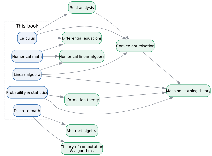
| Subject | What it is and why it matters to you | A good next step |
|---|---|---|
Real analysis |
Calculus done rigorously: what a limit, a real number, continuity and convergence really are. It is where "prove when proof teaches" becomes the main activity, and it underpins every convergence guarantee in optimisation and probability. |
Stephen Abbott, Understanding Analysis. Work the exercises; this is a subject learned by proving. |
Linear algebra, second pass |
Abstract vector spaces, the singular value decomposition, projections and least squares in depth. The SVD alone explains PCA, recommender systems and low-rank approximation of neural networks. |
Gilbert Strang, Introduction to Linear Algebra (and his recorded MIT lectures). |
Convex optimisation |
When problems are convex they can be solved reliably and fast; recognising and formulating convex problems is a superpower in ML, finance, control and operations research. |
Boyd and Vandenberghe, Convex Optimization (freely available from the authors). |
Numerical linear algebra |
How computers actually solve \(A\mathbf{x} = \mathbf{b}\), least squares and eigenproblems at scale: QR, SVD, Krylov methods, conditioning and stability. The engine room under NumPy, SciPy and every ML library. |
Trefethen and Bau, Numerical Linear Algebra. |
Probability and statistics, second pass |
Measure-free but rigorous probability, Bayesian inference, and statistical learning theory. |
Blitzstein and Hwang, Introduction to Probability; then Hastie, Tibshirani and Friedman, The Elements of Statistical Learning (free online). |
Information theory |
Entropy, coding, channel capacity, and their deep links to inference and learning. |
David MacKay, Information Theory, Inference, and Learning Algorithms (free online); Cover and Thomas for depth. |
Machine learning |
The modern synthesis of everything in this chapter. |
Bishop, Pattern Recognition and Machine Learning; Goodfellow, Bengio and Courville, Deep Learning (free online). |
Differential equations and dynamical systems |
How systems evolve: physics, biology, epidemics, control, and the continuous-time view of optimisation. |
Steven Strogatz, Nonlinear Dynamics and Chaos — unusually readable and full of applications. |
Abstract algebra |
Groups, rings and fields: the mathematics of symmetry, and the foundation of cryptography and error-correcting codes (building on Chapter 23). |
Charles Pinter, A Book of Abstract Algebra. |
Theory of computation and algorithms |
Automata, computability, complexity, and the analysis of algorithms, built on Chapter 21, Chapter 22, Chapter 24 and Chapter 25. |
Sipser, Introduction to the Theory of Computation; Cormen et al., Introduction to Algorithms. |
How to choose. Follow your projects. If you work on search, go to information theory and numerical linear algebra. If you train models, go to convex optimisation and machine learning. If you found yourself enjoying the proofs in Chapter 22 and Chapter 23, go to real analysis or abstract algebra. Whatever you choose, keep the habit this book has tried to build: understand → calculate by hand → implement → experiment, and keep asking when should I use this, and when shouldn’t I?
33.9. Reading mathematics
The success criterion for this book was never "can execute procedures". It was this: when you see a formula in a paper, you can unpack it — say what each symbol means, what the whole thing computes, why it has that shape, and how you would implement it. This final section practises exactly that on formulas you will genuinely meet in machine-learning and information-retrieval papers.
Input: an unfamiliar formula in a paper.
Steps:
-
Find the type of the result. Is the left-hand side a number, a vector, a probability, a function, a set? Is this a definition (often \(:=\) or \(\equiv\)), an equation to solve, or an update rule (\(\leftarrow\) or a subscript \(t+1\))?
-
List every symbol and look up any you do not know — most papers define them in the preceding paragraph or in a notation section. Note which are data, which are parameters, and which are dummy (bound) variables such as summation indices.
-
Identify the big operators (\(\sum\), \(\prod\), \(\mathbb{E}\), \(\operatorname{argmin}\), \(\nabla\)) and their scope: what they range over and what they apply to.
-
Read it aloud in words, from the outside in.
-
Make it concrete: plug in tiny numbers (two dimensions, three data points) and compute by hand.
-
Sketch the code: loops for sums,
max/argmaxfor optimisation, matrix products for vectors.
Output: a plain-language explanation and an implementation sketch.
33.9.1. 1. The gradient: \(\nabla f(\mathbf{x})\)
| Symbol | Meaning |
|---|---|
\(f\) |
a scalar-valued function of several variables, for example a loss |
\(\mathbf{x}\) |
bold: a vector, the point \((x_1, \dots, x_n)\) at which we evaluate |
\(\nabla\) |
"nabla" or "del": the gradient operator |
\(\partial f / \partial x_i\) |
partial derivative: rate of change of \(f\) when only \(x_i\) moves |
\({}^{\mathsf T}\) |
transpose: write the row as a column |
In words: "the gradient of \(f\) at \(\mathbf{x}\)" is the vector of partial derivatives. It points in the direction of steepest increase of \(f\), its length is that steepest rate, and it is perpendicular to the contour through \(\mathbf{x}\). Optimisation algorithms step in the direction \(-\nabla f(\mathbf{x})\) to decrease \(f\) — which is why papers write update rules like \(\theta_{t+1} = \theta_t - \eta\nabla_\theta L(\theta_t)\), where the subscript on \(\nabla_\theta\) says "with respect to the parameters \(\theta\), not the data". Concretely: for \(f(x, y) = x^2 + 3y\), \(\nabla f = (2x, 3)\), and at \((1, 2)\) it is \((2, 3)\). Code: by hand, or loss.backward() and read .grad.
33.9.2. 2. Relevance as a dot product: \(\mathbf{q}\cdot\mathbf{d}\)
| Symbol | Meaning |
|---|---|
\(s(\cdot,\cdot)\) |
a score function: two inputs, one number out |
\(\mathbf{q}, \mathbf{d}\) |
query and document vectors in \(\mathbb{R}^k\) (TF-IDF or learned embeddings) |
\(\cdot\) or \(\mathbf{q}^{\mathsf T}\mathbf{d}\) |
the dot product; the second form treats vectors as columns and uses a matrix product |
\(q_j, d_j\) |
the \(j\)-th components |
In words: multiply matching components and add. Geometrically it is \(\lVert\mathbf{q}\rVert\lVert\mathbf{d}\rVert\cos\theta\); if the paper says vectors are normalised, it is the cosine similarity. Ranking all documents means computing \(D\mathbf{q}\) for a matrix \(D\) whose rows are documents, then sorting. Code: scores = D @ q; top = np.argsort(-scores)[:10].
33.9.3. 3. Conditional probability and Bayes: \(P(A \mid B)\)
| Symbol | Meaning |
|---|---|
\(P(\cdot)\) |
probability of an event |
\(\mid\) |
"given": restrict attention to outcomes where the right-hand event happened |
\(A \cap B\) |
"A and B": both events happen |
\(P(A)\) |
the prior: belief in \(A\) before seeing evidence |
\(P(B \mid A)\) |
the likelihood: how probable the evidence is if \(A\) is true |
In words: conditioning on \(B\) means shrinking the universe to the outcomes where \(B\) happened and re-normalising, which is why we divide by \(P(B)\). Bayes' theorem follows from writing \(P(A \cap B)\) two ways: \(P(A \mid B)P(B) = P(B \mid A)P(A)\). Concretely: a disease with prevalence 1% and a test that is 99% sensitive with a 5% false-positive rate gives \(P(\text{ill} \mid +) = \frac{0.99 \times 0.01}{0.99 \times 0.01 + 0.05 \times 0.99} = \frac{0.0099}{0.0594} \approx 0.167\) — only one positive in six is truly ill (Chapter 29). In ML papers, \(p(y \mid \mathbf{x}; \theta)\) means "the model’s probability of label \(y\) given input \(\mathbf{x}\)", with the semicolon separating the parameters \(\theta\) from the conditioning.
33.9.4. 4. Training as optimisation: \(\operatorname{argmin}\)
| Symbol | Meaning |
|---|---|
\(\hat\theta\) |
"theta-hat": the estimated parameters (hats mark estimates) |
\(\operatorname{argmin}_{\theta\in\Theta}\) |
the value of \(\theta\), ranging over the allowed set \(\Theta\), that minimises what follows |
\(f_\theta\) |
the model, a function whose behaviour depends on \(\theta\) |
\((\mathbf{x}_i, y_i)\) |
the \(i\)-th training example: input and label |
\(\ell(\cdot,\cdot)\) |
the per-example loss, such as squared error or cross-entropy |
\(\lambda\lVert\theta\rVert_2^2\) |
regularisation: \(\lambda\) times the sum of squared parameters (the subscript 2 means the ordinary Euclidean norm) |
In words: "the estimated parameters are those, among the allowed ones, that minimise the average training loss plus a penalty on large weights." That one line describes ridge regression, regularised logistic regression and (with a neural-network \(f_\theta\)) most of deep learning. The formula says what is computed, not how: the how is the normal equations, gradient descent or Adam (Section 33.1). Code: the training loop.
33.9.5. 5. Expectation: \(\mathbb{E}[X]\)
| Symbol | Meaning |
|---|---|
\(\mathcal{L}\) |
calligraphic L: a loss (papers use fancy fonts to distinguish objects) |
\(\mathbb{E}[\cdot]\) |
expected value: the probability-weighted average (Chapter 29) |
\((\mathbf{x}, y) \sim \mathcal{D}\) |
"drawn from" the data distribution \(\mathcal{D}\); the subscript says what is random |
\(-\log p_\theta(y \mid \mathbf{x})\) |
the surprise of the true label under the model: cross-entropy for one example |
In words: "the loss is the average surprise of the true label, averaged over all the data the world could give us." We cannot compute an expectation over the whole world, so we estimate it with an average over the training set, \(\frac1n\sum_i -\log p_\theta(y_i \mid \mathbf{x}_i)\), and SGD estimates that with a mini-batch. Recognising "expectation, estimated by an average" is half of reading ML theory. For a discrete random variable, \(\mathbb{E}[X] = \sum_x x\,P(X = x)\); a fair die has \(\mathbb{E}[X] = (1 + 2 + \dots + 6)/6 = 3.5\).
33.9.6. 6. Softmax: turning scores into probabilities
Try it: Softmax with a temperature.
| Symbol | Meaning |
|---|---|
\(\mathbf{z}\) |
a vector of \(K\) real-valued scores ("logits"), one per class |
\(\operatorname{softmax}(\mathbf{z})_i\) |
the \(i\)-th component of the output vector |
\(e^{z_i}\) |
exponentiate: makes every score positive and exaggerates differences |
\(\sum_j e^{z_j}\) |
the normaliser, so the outputs sum to 1 |
In words: "exponentiate each score and divide by the total." The output is a probability distribution over \(K\) classes, with the largest score getting the largest probability — a "soft" version of picking the maximum. With \(K = 2\) it reduces to the sigmoid: \(\frac{e^{z_1}}{e^{z_1} + e^{z_2}} = \sigma(z_1 - z_2)\). Adding the same constant to every score changes nothing (it cancels top and bottom), which is the key to computing it safely:
import math

def softmax(z):
    m = max(z)                          # subtract the max for numerical safety
    exps = [math.exp(zi - m) for zi in z]
    total = sum(exps)
    return [e / total for e in exps]

scores = [2.0, 1.0, 0.1]
print([round(p, 3) for p in softmax(scores)])
print([round(p, 3) for p in softmax([1000.0, 999.0, 998.1])])  # same gaps, no overflow
[0.659, 0.242, 0.099] [0.659, 0.242, 0.099]
Without the subtraction, \(e^{1000}\) overflows to infinity (Chapter 32). By hand for the first case: \(e^{2} \approx 7.389\), \(e^{1} \approx 2.718\), \(e^{0.1} \approx 1.105\), total \(\approx 11.212\), giving \(7.389/11.212 \approx 0.659\), and so on.
33.9.7. 7. A final boss: attention
Here is the formula at the heart of the transformer architecture behind modern language models. You now have every piece: Try it: Attention, step by step.
-
\(Q\), \(K\), \(V\) are matrices whose rows are query, key and value vectors — one per token, produced by linear layers.
-
\(QK^{\mathsf T}\) is a matrix of dot products: entry \((i, j)\) is \(\mathbf{q}_i\cdot\mathbf{k}_j\), "how relevant is token \(j\) to token \(i\)?" — exactly the retrieval score from Section 33.5.
-
Dividing by \(\sqrt{d_k}\) (the vector dimension) keeps the dot products from growing with dimension, so the softmax does not saturate and kill the gradients (the vanishing-gradient worry from Section 33.4).
-
\(\operatorname{softmax}\) is applied to each row, turning relevance scores into weights that sum to 1.
-
Multiplying by \(V\) takes, for each token, a weighted average of the value vectors.
In words: "each token looks up every other token by dot-product similarity, and takes a probability-weighted average of what it finds." A search engine, a softmax and a matrix product — three ideas from this book — make up one line of the most influential formula in current computing.
|
Notation is a compression scheme
Much of the notation you have learned is surprisingly young. Leibniz introduced \(\int\) and \(dx\) in the 1670s; Euler popularised \(\sum\), \(f(x)\), \(e\) and \(\pi\) in the 1700s; the nabla \(\nabla\) was named in the 1800s after a Hebrew harp of that shape; and blackboard-bold \(\mathbb{E}\) for expectation became common only in the 20th century. Good notation is, in Shannon’s sense, a compression scheme: it spends few symbols on the ideas that recur most often. That is why it looks dense — and why, once you know the code, it reads fast. |
|
Formula decoder
Paste a LaTeX formula. Hover over any symbol to see its name, its meaning, and the chapter of this book that introduced it. Then switch to "concrete mode": the lab asks for tiny example values, evaluates the formula step by step, and shows equivalent NumPy code. |
33.10. Interactive tools
Browser tools on the companion website that go with this chapter. Each example link in the chapter opens one of them with that example already set up.
33.11. Mastery check
-
Explain in words what \(\nabla f(\mathbf{x})\) is, what direction it points, and how gradient descent uses it. For \(f(x, y) = x^2 + xy\), compute \(\nabla f(1, 2)\) and one gradient-descent step from \((1, 2)\) with \(\eta = 0.1\).
-
Why is it significant that the least-squares and logistic-regression losses are convex, while neural-network losses are not?
-
Fit the least-squares line to \((0, 0), (1, 1), (2, 3)\) using the normal equations.
-
A logistic-regression model has \(w = 2\), \(b = -4\). What is the predicted probability at \(x = 2\)? At \(x = 3\)? Where is the decision boundary?
-
For one neuron \(a = \sigma(wx + b)\) with loss \(L = (a - y)^2\), write \(\partial L/\partial b\) as a product of three factors from the chain rule.
-
Vectors \(\mathbf{q} = (3, 4)\) and \(\mathbf{d} = (4, 3)\): compute \(\mathbf{q}\cdot\mathbf{d}\) and the cosine similarity.
-
Compute the entropy of a source with probabilities \((\tfrac14, \tfrac14, \tfrac14, \tfrac14)\) and of \((\tfrac12, \tfrac12, 0, 0)\). Which is more compressible?
-
Decode, in words, \(\hat\theta = \operatorname*{argmin}_\theta \mathbb{E}_{(\mathbf{x},y)\sim\mathcal{D}}[-\log \operatorname{softmax}(f_\theta(\mathbf{x}))_y]\).
Decision rule: All correct without hesitation → you have finished the book; choose a horizon from Section 33.8 and go. Stuck on 1–2 → reread the relevant section (Section 33.1, Section 33.2, Section 33.3, Section 33.4, Section 33.5, Section 33.6, or Section 33.9). Stuck on more → revisit the foundations this chapter leans on: Chapter 20, Chapter 26 and Chapter 29.
Mastery check answers
-
The gradient is the vector of partial derivatives of \(f\) at \(\mathbf{x}\); it points in the direction of steepest increase, and gradient descent steps the opposite way, \(\mathbf{x} \leftarrow \mathbf{x} - \eta\nabla f(\mathbf{x})\). Here \(\nabla f = (2x + y,\ x)\), so \(\nabla f(1, 2) = (4, 1)\), and the step gives \((1, 2) - 0.1(4, 1) = (0.6,\ 1.9)\).
-
For a convex loss every local minimum is global, so gradient descent (or the normal equations) is guaranteed to find the best parameters regardless of the starting point. For non-convex losses there may be many local minima and saddle points; the result depends on initialisation and the optimiser, and there is no guarantee of optimality.
-
\(n = 3\), \(\sum x = 3\), \(\sum y = 4\), \(\sum x^2 = 5\), \(\sum xy = 0 + 1 + 6 = 7\). Equations: \(4 = 3b + 3w\) and \(7 = 3b + 5w\). Subtract: \(3 = 2w\), so \(w = 1.5\); then \(3b = 4 - 4.5 = -0.5\), so \(b = -1/6 \approx -0.167\). Line: \(\hat y = 1.5x - 1/6\).
-
At \(x = 2\): \(z = 0\), \(p = \sigma(0) = 0.5\). At \(x = 3\): \(z = 2\), \(p = \sigma(2) \approx 0.881\). The boundary is where \(z = 0\): \(x = -b/w = 2\).
-
\(\dfrac{\partial L}{\partial b} = \dfrac{\partial L}{\partial a}\cdot\dfrac{\partial a}{\partial z}\cdot\dfrac{\partial z}{\partial b} = 2(a - y)\cdot a(1 - a)\cdot 1\).
-
\(\mathbf{q}\cdot\mathbf{d} = 12 + 12 = 24\); both norms are 5, so \(\cos\theta = 24/25 = 0.96\).
-
Uniform over four: \(\log_2 4 = 2\) bits. \((\tfrac12, \tfrac12, 0, 0)\): 1 bit (the zero-probability symbols contribute nothing). The second has lower entropy and is more compressible: 1 bit per symbol instead of 2.
-
"The estimated parameters are those that minimise the expected cross-entropy: over examples drawn from the data distribution, the model turns its output scores into class probabilities with a softmax, and we penalise the negative log-probability (the surprise) of the true class \(y\)." In practice the expectation is replaced by an average over training data and minimised with SGD; this one line is the training objective of essentially every multi-class classifier, including next-token prediction in language models.