Volume 2: Continuous Mathematics · Part V: Calculus
Chapter 17. The Derivative
Chapter map: we start with a car and a stopwatch and ask what "speed at an instant" can possibly mean. Chasing that question turns average rates of change into a limit, and the limit is the derivative. Only once the idea exists do we build the machinery: computing derivatives from first principles, deriving the power, product, quotient and chain rules, finding the derivatives of sine, cosine, \(e^x\) and \(\ln x\), differentiating implicitly, and taking second and higher derivatives. We finish by asking where derivatives fail to exist, and how computers actually compute them, numerically, with dual numbers, and by backpropagation, which turns out to be nothing but the chain rule.
Why this chapter matters: almost every question of the form "how fast?" or "how sensitive?" is a derivative. How fast is the coffee cooling, how much does one extra unit cost to make, how quickly is the ladder sliding, which way should each of a billion neural-network weights move to reduce the error? Speedometers, physics engines, economists' "marginal" anything and every machine-learning training loop compute derivatives all day long.
17.1. Instantaneous speed: the problem
17.1.1. The problem
A car is travelling along a straight road. You have its odometer reading at every moment. Between 2:00 and 2:30 it covered 30 miles. Its average speed over that half-hour was
That is uncontroversial. Now look at the speedometer. At precisely 2:17:04 the needle points at 63 mph. What does that mean?
Speed is distance divided by time. But at a single instant, no time passes and no distance is covered. The formula gives \(0/0\), which is meaningless. Yet the speedometer is not lying: the car really is going 63 mph "right now". Something about that statement is true, and this chapter is about making it precise.
This was a live philosophical problem for two thousand years (Zeno’s arrow paradox is a version of it). Newton and Leibniz resolved it in the 1660s–1680s, and the resolution is the derivative.
|
Rate of change and the symbol \(\Delta\)
The Greek capital delta, \(\Delta\), means "change in". If a quantity goes from \(d_1\) to \(d_2\), then \(\Delta d = d_2 - d_1\). It is a single symbol: \(\Delta t\) is not \(\Delta \times t\). The average rate of change of \(d\) with respect to \(t\) over an interval is \(\dfrac{\Delta d}{\Delta t}\). For distance against time this is average speed; for any function it is the slope of the straight line joining the two endpoints of the graph. |
17.1.2. Intuition: shrink the interval
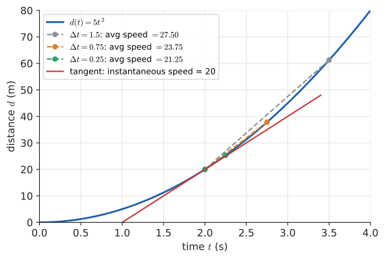
We can’t divide by zero time, but we can divide by small times. Let a ball roll down a ramp so that its distance (metres) after \(t\) seconds is
How fast is it going at exactly \(t = 2\)? Compute the average speed from \(t=2\) to \(t = 2 + \Delta t\) for smaller and smaller \(\Delta t\):
| \(\Delta t\) | \(d(2+\Delta t)\) | \(\Delta d = d(2+\Delta t) - 20\) | average speed \(\Delta d / \Delta t\) |
|---|---|---|---|
1 |
45 |
25 |
25 |
0.1 |
22.05 |
2.05 |
20.5 |
0.01 |
20.2005 |
0.2005 |
20.05 |
0.001 |
20.020005 |
0.020005 |
20.005 |
The averages are homing in on 20 m/s. And we can see why with algebra instead of a calculator. For any \(\Delta t \neq 0\):
The table is just this formula evaluated at \(\Delta t = 1, 0.1, 0.01, 0.001\). As \(\Delta t \to 0\), the average speed approaches 20. We define the instantaneous speed at \(t=2\) to be that limit:
Notice the trick that dissolves the paradox. We never divide by zero. We divide by small non-zero numbers, simplify while that is legal, and only then ask what happens as the interval shrinks. That is exactly what limits were built for in Chapter 16.
17.2. From secant to tangent
17.2.1. The same idea, drawn
On a distance–time graph, the average speed between two times is the slope of the straight line joining the two points on the curve. The instantaneous speed is the slope of the line that just touches the curve at one point. This picture works for any function, not just motion, so let us name the pieces.
|
Secant line and tangent line
A secant line (from Latin secare, to cut) is a line through two points on a curve. Its slope, \(\dfrac{f(a+h) - f(a)}{h}\), is the average rate of change of \(f\) between \(a\) and \(a+h\). A tangent line (from Latin tangere, to touch) at a point \(P\) is the line through \(P\) whose direction matches the curve’s direction at \(P\). Zoom in far enough on a smooth curve at \(P\) and the curve and its tangent become indistinguishable. Note: the tangent line is unrelated to the trig function \(\tan\) except by shared etymology. |
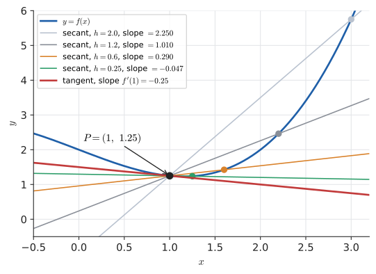
Take \(f(x) = \tfrac14 x^3 - x + 2\) and the point \(P = (1, f(1)) = (1, 1.25)\). The secant from \(P\) to the point at \(x = 1+h\) has slope Try it: Drag the secant to P.
Evaluate for a few values of \(h\): \(h=2\) gives \(2.25\); \(h=1.2\) gives \(1.01\); \(h=0.6\) gives \(0.29\); \(h=0.25\) gives \(-0.046875\). As \(h \to 0\) the slope tends to \(-0.25\), which is the slope of the tangent at \(P\).
|
Secant to tangent
Drag a second point \(Q\) along a curve towards a fixed point \(P\). A readout shows the secant slope to six decimal places as \(h\) shrinks, and a second panel plots secant slope against \(h\). Try a smooth curve, then \(\lvert x \rvert\) at \(P = (0,0)\), and watch the slopes from the left and the right refuse to agree. |
17.3. The definition of the derivative
17.3.1. Formalisation
Everything so far collapses into one definition.
Read it piece by piece:
-
\(f(a+h) - f(a)\) is the change in output, \(\Delta y\), when the input moves from \(a\) to \(a + h\);
-
dividing by \(h\) (which is \(\Delta x\)) gives the average rate of change, the secant slope;
-
\(\lim_{h \to 0}\) asks what that slope approaches as the interval shrinks, without ever setting \(h = 0\);
-
\(f'(a)\), read "f prime of a", is the result: the instantaneous rate of change of \(f\) at \(a\), the slope of the tangent there.
If the limit exists, \(f\) is differentiable at \(a\). If we let \(a\) vary, we get a new function, \(x \mapsto f'(x)\), the derivative of \(f\). Finding it is called differentiation.
|
Derivative, difference quotient, differentiable
The difference quotient is \(\dfrac{f(x+h) - f(x)}{h}\), the slope of a secant. The derivative \(f'(x)\) is the limit of the difference quotient as \(h \to 0\): the slope of the tangent, or the instantaneous rate of change of \(f\). A function is differentiable at \(x\) if that limit exists (as a finite number). It is differentiable (on an interval) if it is differentiable at every point there. Differentiation is the process of finding a derivative. The word comes from Leibniz’s "differences", the tiny changes \(dx\) and \(dy\). |
17.3.2. Notation: four ways to write the same thing
Calculus was invented twice, by Newton and by Leibniz, and both notations survive. You will meet all of these, sometimes in the same paper.
|
Notations for the derivative
Lagrange (prime) notation: \(f'(x)\), \(f''(x)\) for the second derivative. Compact; good when the function has a name. Leibniz notation: if \(y = f(x)\), write \(\dfrac{dy}{dx}\) ("dee y by dee x"). It looks like \(\dfrac{\Delta y}{\Delta x}\) with the deltas made infinitely small, which is exactly the intuition. Value at a point: \(\left.\dfrac{dy}{dx}\right\rvert_{x=a}\). Operator notation: \(\dfrac{d}{dx}\) is an operator: a machine that takes a function and returns its derivative. \(\dfrac{d}{dx}\left(x^2\right) = 2x\) reads "the derivative with respect to \(x\) of \(x^2\) is \(2x\)". Also written \(D_x\) or \(D\). Newton (dot) notation: \(\dot{x}\) for the derivative of \(x\) with respect to time, \(\ddot{x}\) for the second. Common in mechanics and physics. |
Leibniz notation earns its keep because it records which variable you are differentiating with respect to. \(\frac{dV}{dr}\) and \(\frac{dV}{dt}\) are different questions about the same volume \(V\): how fast it changes per unit of radius, versus per second. It also makes the chain rule look like fraction cancellation, which (as we’ll see) is a helpful mnemonic and a dangerous proof.
|
\(dy/dx\) is not (quite) a fraction
\(\frac{dy}{dx}\) is a single symbol meaning a limit of fractions. It is not \(dy\) divided by \(dx\), and you cannot cancel the \(d\)s to get \(\frac{y}{x}\). Leibniz’s notation is designed so that many fraction-like manipulations give correct answers (the chain rule, inverse functions, separation of variables), but each of those is a theorem, not an algebra rule. Similarly \(\frac{d}{dx}\) on its own is an instruction, like a function name waiting for an argument. |
17.3.3. Where you’d use this
Whenever a quantity changes, its derivative is "how fast, right now", and the difference quotient is "how fast, on average". Both show up constantly.
-
Everyday: average versus instantaneous speed. UK average-speed cameras photograph your number plate at two points and divide. Two cameras 2 km apart and a crossing time of 72 s give \(2 \div (72/3600) = 100\) km/h, about 62 mph: a secant slope. A fixed camera with radar measures (very nearly) the derivative. You can drive at 80 mph past the first camera and still average 62; the two measurements answer different questions.
-
Economics: marginal cost. If making \(q\) units costs \(C(q) = 500 + 4q + 0.01q^2\) pounds, the marginal cost is \(C'(q) = 4 + 0.02q\). At \(q = 100\) it is \(C'(100) = 6\) pounds: the cost of one more unit. Check: \(C(101) - C(100) = 6.01\). Economists say "marginal" where mathematicians say "derivative".
-
Science and engineering. Electric current is the rate of flow of charge, \(I = \frac{dQ}{dt}\) (one ampere is one coulomb per second). Reaction rate in chemistry is \(\frac{d[\text{concentration}]}{dt}\). Power is the rate of doing work, \(P = \frac{dW}{dt}\): a kettle that delivers 3 kW turns 3000 joules per second into heat.
-
Computing: rates from counters. Monitoring systems store ever-increasing counters (total requests served) and compute rates from them. Prometheus’s
rate(requests_total[5m])is a secant slope: if the counter went from 12,000 to 15,600 over 300 seconds, the rate is \(3600/300 = 12\) requests per second. Choosing the window is choosing \(h\): a short window is closer to "instantaneous" but noisier, the same trade-off you will meet in Section 17.10.
17.4. Derivatives from first principles
Computing a derivative directly from the limit definition is called working from first principles. You will rarely do it once you have the rules, but doing it a few times is how you come to trust the rules, and it is how we will derive them.
Input: a function \(f\).
Steps:
-
Write the difference quotient \(\dfrac{f(x+h) - f(x)}{h}\).
-
Substitute the formula for \(f\) at both \(x + h\) and \(x\).
-
Simplify algebraically (expand, combine fractions, or multiply by a conjugate) until a factor of \(h\) in the numerator cancels the \(h\) in the denominator. This step is legal because \(h \neq 0\) inside the limit.
-
Now that nothing divides by \(h\), let \(h \to 0\) (usually by substituting \(h = 0\)).
Output: \(f'(x)\).
17.4.1. Worked example: \(f(x) = x^2\)
So the slope of the parabola \(y = x^2\) at \(x\) is \(2x\): zero at the vertex, 2 at \(x = 1\), \(-6\) at \(x = -3\).
17.4.2. Worked example: \(f(x) = x^3\)
17.4.3. Worked example: \(f(x) = \dfrac{1}{x}\)
Here the simplification step is "combine the fractions":
The slope is always negative (the hyperbola always falls) and gets steeper near \(x = 0\).
17.4.4. Worked example: \(f(x) = \sqrt{x}\)
Here the simplification step is the conjugate trick from Chapter 16: multiply top and bottom by \(\sqrt{x+h} + \sqrt{x}\) so that the difference of square roots becomes a difference of squares.
17.4.5. Spot the pattern
Write each function as a power of \(x\):
| \(f(x)\) | as a power | \(f'(x)\) | as a power |
|---|---|---|---|
\(x^2\) |
\(x^2\) |
\(2x\) |
\(2x^1\) |
\(x^3\) |
\(x^3\) |
\(3x^2\) |
\(3x^2\) |
\(1/x\) |
\(x^{-1}\) |
\(-1/x^2\) |
\(-1\cdot x^{-2}\) |
\(\sqrt{x}\) |
\(x^{1/2}\) |
\(1/(2\sqrt{x})\) |
\(\tfrac12 x^{-1/2}\) |
Every time: bring the exponent down in front, then reduce the exponent by one. That is the power rule, \(\frac{d}{dx}x^n = nx^{n-1}\), and we have now earned it rather than been handed it. The next section proves it.
|
Who got there first?
Newton developed his "method of fluxions" around 1665–66, while Cambridge was closed for the plague, but published little of it for decades. Leibniz developed his calculus independently in the 1670s and published first, in 1684. The resulting priority dispute became a national feud; British mathematicians clung to Newton’s dot notation for a century and fell behind the Continent, which used Leibniz’s far more flexible \(dy/dx\). Notation matters. |
17.4.6. Exercises
-
Use the definition to find the slope of the secant to \(f(x) = x^2\) between \(x = 3\) and \(x = 3.1\), then find \(f'(3)\).
-
Differentiate \(f(x) = 4x^2 - 3x + 7\) from first principles.
-
Differentiate \(f(x) = \dfrac{1}{x^2}\) from first principles and check your answer against the power-rule pattern.
Answers
-
Secant slope \(= \dfrac{3.1^2 - 3^2}{0.1} = \dfrac{9.61 - 9}{0.1} = 6.1\). From the worked example, \(f'(x) = 2x\), so \(f'(3) = 6\). (Formula check: secant slope \(= 2x + h = 6 + 0.1\).)
-
\(f(x+h) - f(x) = 4(x^2 + 2xh + h^2) - 3x - 3h + 7 - 4x^2 + 3x - 7 = 8xh + 4h^2 - 3h\). Divide by \(h\): \(8x + 4h - 3\). Let \(h \to 0\): \(f'(x) = 8x - 3\).
-
\(\dfrac{1}{h}\left(\dfrac{1}{(x+h)^2} - \dfrac{1}{x^2}\right) = \dfrac{1}{h}\cdot\dfrac{x^2 - (x+h)^2}{x^2(x+h)^2} = \dfrac{1}{h}\cdot\dfrac{-2xh - h^2}{x^2(x+h)^2} = \dfrac{-2x - h}{x^2(x+h)^2}\). As \(h \to 0\) this tends to \(\dfrac{-2x}{x^4} = -\dfrac{2}{x^3}\), which is \(-2x^{-3}\), exactly \(nx^{n-1}\) with \(n = -2\).
17.5. The rules of differentiation
17.5.1. The problem
First principles works, but try it on \(f(x) = x^7\sin x + \sqrt{1 + x^2}\) and you’ll be at it all afternoon. What we want is a small set of rules, each derived once from the definition, that let us differentiate any formula built from standard pieces by taking it apart. This is exactly how a compiler handles expressions: a handful of rules for the building blocks and the ways of combining them, applied recursively.
The building blocks are powers, exponentials, logs and trig functions. The ways of combining are: multiply by a constant, add, multiply, divide, and compose. We need one rule for each.
17.5.2. Constant, constant multiple and sum rules
Constants. If \(f(x) = c\) then \(f(x+h) - f(x) = c - c = 0\), so \(f'(x) = 0\). A flat line has slope zero.
Constant multiple. If \(g(x) = c\,f(x)\):
Stretching a graph vertically by a factor of \(c\) stretches every slope by \(c\).
Sum. If \(s(x) = f(x) + g(x)\):
Together these say differentiation is linear: \(\frac{d}{dx}(af + bg) = af' + bg'\). That word will mean a great deal in Chapter 27.
17.5.3. The power rule
For a positive whole number \(n\), the binomial theorem (Chapter 7) expands \((x+h)^n\):
The only facts we need: the first term is \(x^n\), the second is \(nx^{n-1}h\), and every remaining term contains at least \(h^2\). So
We proved it for positive integers. It is in fact true for every real exponent \(n\) (we already checked \(n = -1\) and \(n = \tfrac12\) by hand); the general proof comes for free once we have \(\ln x\), later in this chapter.
Worked example. Differentiate \(p(x) = 4x^5 - 3x^2 + \dfrac{2}{x} - 7\sqrt{x} + 9\). Try it: Differentiate it symbolically.
First rewrite every term as a power of \(x\), because the power rule needs that form:
17.5.4. The product rule
The problem. Is the derivative of a product the product of the derivatives? Try \(x \cdot x = x^2\): the product of derivatives is \(1 \cdot 1 = 1\), but the true derivative is \(2x\). So no. Try it: Grow the product-rule rectangle.
Intuition: a growing rectangle. Picture \(f(x)\,g(x)\) as the area of a rectangle with sides \(f\) and \(g\). Nudge \(x\) by \(h\). The width grows by \(\Delta f\) and the height by \(\Delta g\). The area gains three pieces: a strip \(g\,\Delta f\) down the side, a strip \(f\,\Delta g\) across the top, and a tiny corner \(\Delta f\,\Delta g\).
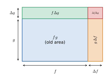
Why it works. Divide the change in area by \(h\):
As \(h \to 0\), \(\frac{\Delta f}{h} \to f'\) and \(\frac{\Delta g}{h} \to g'\), while \(\Delta g \to 0\) (because \(g\) is continuous), so the corner term vanishes:
In words: "derivative of the first times the second, plus the first times derivative of the second". Each factor takes its turn changing while the other is held fixed.
Worked example. \(\dfrac{d}{dx}\left(x^2 \sin x\right)\). Let \(f = x^2\), \(g = \sin x\), so \(f' = 2x\) and \(g' = \cos x\) (proved in the next section): Try it: Differentiate it symbolically.
17.5.5. The quotient rule
Why it works. Let \(Q = f/g\), so \(f = Qg\). Differentiate both sides with the product rule and solve for \(Q'\):
(This derivation assumes \(Q\) is differentiable; a first-principles proof removes that assumption and gives the same formula.) The traditional mnemonic: "low d-high minus high d-low, over the square of what’s below". The order matters because of the minus sign.
Worked example. \(\dfrac{d}{dx}\,\dfrac{x}{x^2 + 1}\). With \(f = x\), \(f' = 1\), \(g = x^2+1\), \(g' = 2x\): Try it: Differentiate it symbolically.
The derivative is zero at \(x = \pm 1\), which is where the graph turns: the maximum value \(\tfrac12\) and minimum \(-\tfrac12\). Finding turning points this way is the subject of Chapter 18.
17.5.6. The chain rule
The problem. How do we differentiate a composition, a function of a function, such as \(\sin(x^2)\) or \((3x^2 + 1)^5\)? Expanding \((3x^2+1)^5\) is possible but miserable; expanding \(\sqrt{1 + x^2}\) is impossible.
Intuition: gears. Three gears are meshed. Gear B turns 3 times for every turn of gear A; gear C turns 2 times for every turn of gear B. How many times does C turn per turn of A? \(3 \times 2 = 6\). Rates of change through a chain multiply.
Now write the composition as a chain. If \(y = (3x^2 + 1)^5\), introduce the inner quantity \(u = 3x^2 + 1\), so \(y = u^5\). Then \(x\) drives \(u\) at rate \(\frac{du}{dx} = 6x\), and \(u\) drives \(y\) at rate \(\frac{dy}{du} = 5u^4\). So \(x\) drives \(y\) at rate
In Leibniz notation the \(du\)s appear to cancel, which makes the rule easy to remember. In Lagrange notation, for \(y = f(g(x))\):
"Derivative of the outer function, evaluated at the inner function, times the derivative of the inner function."
Why it works. Write \(u = g(x)\) and \(\Delta u = g(x+h) - g(x)\). Provided \(\Delta u \neq 0\) for small \(h\):
As \(h \to 0\), \(\Delta u \to 0\) (since \(g\) is continuous), so the first fraction tends to \(f'(u)\) and the second to \(g'(x)\). The proviso "\(\Delta u \neq 0\)" is a genuine gap: for some functions \(\Delta u\) is zero infinitely often near \(x\). The rigorous proof patches it by replacing the first fraction with a function that equals \(f'(u)\) when \(\Delta u = 0\); the result is unchanged. This is the classic case where the intuitive argument is right in spirit and the careful version is a technicality.
Input: a composite expression \(y = f(g(x))\).
Steps:
-
Identify the outer function \(f\) (the last operation you would perform if evaluating on a calculator) and the inner function \(g\) (everything fed into it).
-
Differentiate the outer function, leaving its inside untouched: \(f'(g(x))\).
-
Multiply by the derivative of the inside: \(g'(x)\).
-
If the inside is itself a composition, repeat steps 1–3 on it (each layer contributes one factor).
Output: \(\dfrac{dy}{dx} = f'(g(x))\,g'(x)\).
Worked examples. Try it: Differentiate (3x² + 1)⁵.
|
Forgetting the inner derivative
The single most common calculus error is writing \(\frac{d}{dx}\sin(x^2) = \cos(x^2)\) and stopping. Every layer of a composition contributes a factor. A quick sanity check: if you replace \(x\) by \(2x\), the graph is squeezed horizontally by a factor of 2, so every slope must double. The chain rule’s "times the derivative of the inside" is exactly that factor. Also: \((fg)' \neq f'g'\) and \((f/g)' \neq f'/g'\). Products and quotients have their own rules. |
17.5.7. Where you’d use this
The chain rule is the one you use without noticing, because it is how rates convert between units.
-
Everyday. Your car uses 0.06 litres per kilometre and you are driving at 90 km/h. Fuel per hour is \(\frac{dF}{dt} = \frac{dF}{dx}\cdot\frac{dx}{dt} = 0.06 \times 90 = 5.4\) litres per hour. Every "per" conversion (pence per kWh times kWh per hour, heartbeats per minute times minutes per day) is the chain rule with constant rates; calculus says it still works when the rates vary.
-
Science and engineering: related rates. The balloon exercise below is the template: you know how fast one quantity changes (radius) and want another (volume) linked to it by a formula. Pumping air into a balloon, oil spreading in a circular slick (\(A = \pi r^2\), so \(\frac{dA}{dt} = 2\pi r\frac{dr}{dt}\)), the shadow of a walker under a streetlight: all one chain rule.
-
Computing: animation easing. Animators move objects with "ease-in, ease-out" curves rather than constant speed. A standard one is smoothstep, \(s(t) = 3t^2 - 2t^3\) for \(0 \le t \le 1\). Its derivative \(s'(t) = 6t - 6t^2\) is 0 at both ends (the object starts and stops gently) and peaks at \(s'(0.5) = 1.5\) in the middle. To run a 2-second animation you use \(s(t/2)\), and the chain rule tells you its speed is \(\tfrac12 s'(t/2)\). The product rule, meanwhile, is behind every "growth of a product" question: revenue = price \(\times\) quantity, so \(R' = p'q + pq'\), which is why a price rise that cuts sales can still lose money.
17.5.8. Choosing a method
You will often have a choice of route. Some guidance:
-
Simplify first. \(\dfrac{x^2 + 1}{x}\) can be done with the quotient rule, but rewriting as \(x + x^{-1}\) gives \(1 - x^{-2}\) in one line.
-
Constant denominators are not quotients. \(\dfrac{x^3}{6}\) is \(\tfrac16 x^3\); derivative \(\tfrac12 x^2\). Using the quotient rule works but invites errors.
-
Roots and reciprocals become powers. \(\dfrac{1}{\sqrt{x}} = x^{-1/2}\), derivative \(-\tfrac12 x^{-3/2}\).
-
Quotient rule versus product-plus-chain. \(\dfrac{f}{g} = f\cdot g^{-1}\); some people never use the quotient rule at all and instead apply the product rule and chain rule to \(f\cdot g^{-1}\). Both are correct; the quotient rule’s formula is usually tidier.
-
Logarithmic differentiation (take \(\ln\) of both sides, then differentiate implicitly) is best for messy products of powers like \(x^x\) or \(\dfrac{(x+1)^3\sqrt{x-2}}{(x^2+5)^4}\). See the exercises below.
|
Rules of differentiation
|
17.5.9. Exercises
-
Differentiate \(y = 6x^4 - \dfrac{3}{x^3} + 5\sqrt[3]{x}\).
-
Differentiate \(y = (2x - 1)(x^3 + 4)\) twice: once with the product rule and once by expanding first. Confirm they agree.
-
Differentiate \(y = \dfrac{x^2}{x - 3}\).
-
Differentiate \(y = (x^2 - 5x)^{10}\) and \(y = \dfrac{1}{(4 - x^2)^3}\).
-
A spherical balloon’s volume is \(V = \tfrac43\pi r^3\), and its radius grows as \(r(t) = 1 + 0.5t\) cm. Use the chain rule to find \(\frac{dV}{dt}\) at \(t = 2\) s.
Answers
-
Rewrite: \(y = 6x^4 - 3x^{-3} + 5x^{1/3}\). Then \(y' = 24x^3 + 9x^{-4} + \tfrac53 x^{-2/3} = 24x^3 + \dfrac{9}{x^4} + \dfrac{5}{3\sqrt[3]{x^2}}\).
-
Product rule: \(2(x^3 + 4) + (2x-1)\cdot 3x^2 = 2x^3 + 8 + 6x^3 - 3x^2 = 8x^3 - 3x^2 + 8\). Expanding: \(y = 2x^4 - x^3 + 8x - 4\), so \(y' = 8x^3 - 3x^2 + 8\). They agree.
-
Quotient rule with \(f = x^2, f' = 2x, g = x - 3, g' = 1\): \(y' = \dfrac{2x(x-3) - x^2}{(x-3)^2} = \dfrac{x^2 - 6x}{(x-3)^2} = \dfrac{x(x-6)}{(x-3)^2}\).
-
\(10(x^2 - 5x)^9(2x - 5)\). For the second, write \((4 - x^2)^{-3}\): derivative \(-3(4-x^2)^{-4}\cdot(-2x) = \dfrac{6x}{(4 - x^2)^4}\).
-
\(\frac{dV}{dr} = 4\pi r^2\), \(\frac{dr}{dt} = 0.5\). At \(t = 2\), \(r = 2\), so \(\frac{dV}{dt} = 4\pi(2)^2(0.5) = 8\pi \approx 25.1\) cm³/s.
17.6. Derivatives of sine, cosine, \(e^x\) and \(\ln x\)
17.6.1. Sine and cosine
Intuition first. Look at the graph of \(\sin x\) and read off its slope. At \(x=0\) it rises steeply (slope 1). At \(x = \pi/2\), the peak, the slope is 0. At \(x = \pi\) it falls as steeply as it rose (slope \(-1\)). At \(3\pi/2\) it bottoms out (slope 0). Plot those slopes and you get \(1, 0, -1, 0, 1, \dots\): the cosine curve.
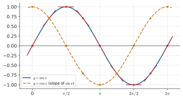
Why it works. We need two limits established in Chapter 16 (with \(h\) in radians): Try it: Build cos x from slopes.
and the addition formula \(\sin(x + h) = \sin x\cos h + \cos x\sin h\) from Chapter 13. Then
The same computation with \(\cos(x+h) = \cos x\cos h - \sin x\sin h\) gives
From these two and the quotient rule, \(\tan x = \sin x/\cos x\) gives
|
Radians, always
\(\frac{d}{dx}\sin x = \cos x\) is true only when \(x\) is measured in radians. The limit \(\frac{\sin h}{h} \to 1\) depends on it. If \(x\) is in degrees, \(\sin(x^\circ) = \sin\!\left(\frac{\pi x}{180}\right)\) and the chain rule gives \(\frac{d}{dx}\sin(x^\circ) = \frac{\pi}{180}\cos(x^\circ)\), an ugly constant that radians exist to eliminate. In calculus, and in every programming language’s |
17.6.2. The exponential function \(e^x\)
The problem. What is the derivative of an exponential \(b^x\)? Start from the definition and use an exponent law:
So the derivative of any exponential is proportional to itself. The constant of proportionality, call it \(M(b) = \lim_{h\to0}(b^h - 1)/h\), is the slope of \(b^x\) at \(x = 0\). Numerically: Try it: Slope of 2ˣ at 0.
| \(h\) | \(b = 2\) | \(b = e \approx 2.71828\) | \(b = 3\) |
|---|---|---|---|
0.1 |
0.71773 |
1.05171 |
1.16123 |
0.01 |
0.69556 |
1.00502 |
1.10467 |
0.001 |
0.69339 |
1.00050 |
1.09922 |
0.0001 |
0.69317 |
1.00005 |
1.09867 |
For base 2 the slope at 0 is about 0.693; for base 3 it is about 1.099. Somewhere between 2 and 3 is the base whose slope at 0 is exactly 1. That base is \(e = 2.71828\ldots\), and for it
This is arguably the best definition of \(e\): the base for which the exponential function is its own derivative. The compound-interest definition \(e = \lim_{n\to\infty}(1 + 1/n)^n\) from Chapter 12 picks out the same number; showing they agree is a nice exercise in limits.
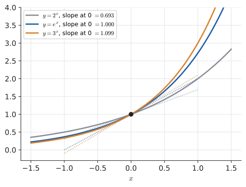
With the chain rule, \(\frac{d}{dx}e^{kx} = k\,e^{kx}\) and \(\frac{d}{dx}e^{g(x)} = g'(x)\,e^{g(x)}\). For example \(\frac{d}{dx}e^{-x^2/2} = -x\,e^{-x^2/2}\): this is the bell curve of Chapter 30, and its slope formula tells you it rises for \(x < 0\) and falls for \(x > 0\). Try it: Slope of eˣ at 0.
|
Why it matters that \(e^x\) is its own derivative
"Rate of growth proportional to current size" describes populations, compound interest, radioactive decay, cooling coffee, charging capacitors and unchecked epidemics. In symbols, \(\frac{dy}{dt} = ky\). We have just shown \(y = Ce^{kt}\) solves it, since \(\frac{d}{dt}Ce^{kt} = kCe^{kt} = ky\). It turns out to be the only solution, which is why \(e\) turns up wherever things grow or decay. This is your first differential equation; Chapter 19 returns to them. |
17.6.3. The natural logarithm \(\ln x\)
\(\ln x\) is the inverse of \(e^x\): \(y = \ln x\) means exactly \(e^y = x\). We know how to differentiate \(e^y\), so differentiate both sides of \(e^y = x\) with respect to \(x\), treating \(y\) as a function of \(x\) and using the chain rule on the left:
Geometrically: the graph of \(\ln\) is the graph of \(\exp\) reflected in the line \(y = x\). Reflection swaps rise and run, so slopes become reciprocals. Where \(e^y\) has slope \(e^y = x\), \(\ln x\) has slope \(1/x\).
Two dividends follow immediately.
Any base. Since \(b = e^{\ln b}\), we have \(b^x = e^{x\ln b}\), and the chain rule gives
So the mysterious constant \(M(b)\) in the table was \(\ln b\) all along: \(\ln 2 = 0.6931\ldots\), \(\ln 3 = 1.0986\ldots\). Similarly \(\frac{d}{dx}\log_b x = \frac{1}{x\ln b}\).
The power rule for every real exponent. For \(x > 0\), \(x^n = e^{n\ln x}\), so
This closes the gap left earlier: \(\frac{d}{dx}x^\pi = \pi x^{\pi - 1}\) is now proved.
|
Standard derivatives
(Angles in radians. The \(\arctan\) entry is derived in the next section.) |
17.6.4. Where you’d use this
-
Everyday: cooling coffee. A cup at 90 °C in a 20 °C room cools roughly as \(T(t) = 20 + 70e^{-0.1t}\) (\(t\) in minutes). Then \(T'(t) = -7e^{-0.1t}\): it is losing 7 °C per minute when poured, but only \(7/e \approx 2.6\) °C per minute ten minutes later. The same formula shape describes a drug washing out of the bloodstream and a capacitor discharging.
-
Engineering: mains electricity. UK mains voltage is \(V(t) = 325\sin(100\pi t)\) volts (230 V rms, 50 Hz). Its rate of change is \(V'(t) = 325 \cdot 100\pi\cos(100\pi t)\), peaking at about \(102{,}000\) volts per second as the voltage crosses zero. Capacitors pass current in proportion to \(\frac{dV}{dt}\), which is why they block steady DC but conduct AC.
-
Finance. £1000 growing at 5% compounded continuously is \(A(t) = 1000e^{0.05t}\), and \(A'(t) = 0.05A(t)\): the balance grows at £50 a year at the start and faster as it grows. "Rate proportional to size" is exactly \(\frac{d}{dt}e^{kt} = ke^{kt}\).
-
Computing: the sigmoid and log-loss. The logistic function \(\sigma(x) = 1/(1 + e^{-x})\), used to turn a score into a probability in logistic regression and neural networks, has the famously convenient derivative \(\sigma'(x) = \sigma(x)(1 - \sigma(x))\) (a chain-rule exercise). At \(x = 0\), \(\sigma = 0.5\) and the slope is \(0.25\). The log in the cross-entropy loss contributes the \(\frac{1}{x}\) from \(\frac{d}{dx}\ln x\); together they make the gradient of the loss with respect to the score simply "prediction minus truth".
17.7. Implicit differentiation
17.7.1. The problem
The circle \(x^2 + y^2 = 25\) has a perfectly good tangent at \((3, 4)\). What is its slope? The trouble is that the circle is not the graph of a single function: solving gives \(y = \pm\sqrt{25 - x^2}\), two functions glued together. For curves like \(x^3 + y^3 = 6xy\) there is no convenient formula for \(y\) at all.
17.7.2. The idea
We don’t need a formula for \(y\). Near any point where the curve is smooth, it locally looks like the graph of some function \(y(x)\), even if we can’t write it down. So differentiate the equation as it stands, treating \(y\) as an unknown function of \(x\). Each time you differentiate an expression in \(y\), the chain rule produces a factor \(\frac{dy}{dx}\); for example \(\frac{d}{dx}y^2 = 2y\frac{dy}{dx}\). Then solve the resulting equation for \(\frac{dy}{dx}\).
|
Implicit and explicit
A function is given explicitly when \(y\) is isolated: \(y = \sqrt{25 - x^2}\). It is given implicitly by an equation relating \(x\) and \(y\) without isolating either: \(x^2 + y^2 = 25\). Implicit differentiation finds \(dy/dx\) directly from the implicit equation. |
Input: an equation in \(x\) and \(y\); optionally a point \((x_0, y_0)\) on the curve.
Steps:
-
Differentiate both sides with respect to \(x\). Treat \(y\) as a function of \(x\): every term containing \(y\) gets a factor \(y' = \frac{dy}{dx}\) from the chain rule, and products like \(xy\) need the product rule.
-
Collect all terms containing \(y'\) on one side, everything else on the other.
-
Factor out \(y'\) and divide.
-
If a point was given, substitute it (check first that it really lies on the curve).
Output: \(y'\) as an expression in \(x\) and \(y\), or its value at the point.
17.7.3. Worked example: the circle
At \((3, 4)\): \(y' = -\tfrac34\). Check against geometry: the radius to \((3,4)\) has slope \(\tfrac43\), and a tangent to a circle is perpendicular to the radius, so its slope is the negative reciprocal, \(-\tfrac34\). Correct. At \((3, -4)\) the same formula gives \(+\tfrac34\), automatically handling the lower half.
17.7.4. Worked example: the folium of Descartes
Find the slope of \(x^3 + y^3 = 6xy\) at \((3, 3)\). First check the point: \(27 + 27 = 54 = 6\cdot 3\cdot 3\). Good.
At \((3,3)\): \(y' = \dfrac{6 - 9}{9 - 6} = -1\).
17.7.5. Worked example: derivative of \(\arctan x\)
Inverse functions are the other big use. \(y = \arctan x\) means \(\tan y = x\) with \(-\tfrac{\pi}{2} < y < \tfrac{\pi}{2}\): Try it: Differentiate arctan x.
A neat surprise: a trig-flavoured function whose derivative is a plain rational function. It is why \(\pi\) appears in \(\int_{-\infty}^{\infty}\frac{dx}{1+x^2} = \pi\).
|
Implicit differentiation needs a smooth point
The formula \(y' = -x/y\) fails at \((5, 0)\), where the circle’s tangent is vertical: the denominator is zero. Implicit differentiation assumes the curve is locally a function graph near the point; where the tangent is vertical or the curve crosses itself (the folium does, at the origin, where the formula gives \(0/0\)), the method’s answer is undefined and you must look at the geometry. The theorem that says when it works is the implicit function theorem, which you’ll meet if you continue into Chapter 20. |
17.7.6. Where you’d use this
-
Everyday and physics: the bicycle pump. Squeeze air slowly (at constant temperature) and Boyle’s law says \(PV\) stays constant, say \(PV = 100\) (kPa and litres). You never need \(P\) as a formula in \(t\): differentiate the constraint with respect to time, \(V\frac{dP}{dt} + P\frac{dV}{dt} = 0\). When \(V = 0.5\) L, \(P = 200\) kPa, and you are compressing at \(\frac{dV}{dt} = -0.1\) L/s, the pressure is rising at \(\frac{dP}{dt} = -\frac{P}{V}\frac{dV}{dt} = -\frac{200}{0.5}(-0.1) = 40\) kPa/s. This is the technique of related rates, worked in detail (ladders, balloons, radar) in Section 18.5.
-
Science: constraints. Orbits, chemical equilibria, and any "these quantities are locked together by an equation" situation are handled the same way: differentiate the constraint, not a solved formula.
-
Computing: implicit shapes. Games and ray tracers often describe surfaces implicitly (a sphere is \(x^2 + y^2 + z^2 = r^2\); signed-distance-field renderers build whole scenes this way). The tangent and normal at a hit point, which drive lighting and how a ball bounces off a curved bumper, come from differentiating the implicit equation, exactly as for the circle above (the multivariable version, the gradient, is in Chapter 20).
17.7.7. Exercises
-
Find \(dy/dx\) for \(x^2 y + y^3 = 10\), and its value at \((3, 1)\).
-
Use logarithmic differentiation to find the derivative of \(y = x^x\) for \(x > 0\). (Take \(\ln\) of both sides first.)
-
Find the slope of the ellipse \(4x^2 + 9y^2 = 72\) at \((3, 2)\).
Answers
-
Check: \(9 + 1 = 10\). Differentiate: \(2xy + x^2 y' + 3y^2 y' = 0\), so \(y'(x^2 + 3y^2) = -2xy\) and \(y' = \dfrac{-2xy}{x^2 + 3y^2}\). At \((3,1)\): \(\dfrac{-6}{9 + 3} = -\tfrac12\).
-
\(\ln y = x\ln x\). Differentiate: \(\dfrac{y'}{y} = \ln x + x\cdot\dfrac1x = \ln x + 1\). So \(y' = x^x(\ln x + 1)\). (Neither the power rule nor the exponential rule applies: the variable is in both base and exponent.)
-
Check: \(36 + 36 = 72\). \(8x + 18y\,y' = 0\), so \(y' = -\dfrac{8x}{18y} = -\dfrac{4x}{9y}\). At \((3,2)\): \(-\dfrac{12}{18} = -\tfrac23\).
17.8. Higher derivatives: velocity, acceleration and beyond
17.8.1. The problem
The derivative of a function is itself a function, so we can differentiate it. Does that mean anything? In mechanics it means a great deal. If \(s(t)\) is position, then \(s'(t)\) is velocity, and the rate of change of velocity is acceleration: the quantity in Newton’s second law, \(F = ma\).
|
Higher derivatives
The second derivative is the derivative of the derivative: \(f''(x)\), or \(\dfrac{d^2y}{dx^2}\) ("dee two y by dee x squared"), or \(\ddot{s}\) in mechanics. The Leibniz form comes from applying the operator twice: \(\frac{d}{dx}\left(\frac{dy}{dx}\right)\). The \(n\)th derivative is written \(f^{(n)}(x)\) (parentheses, so it is not mistaken for a power) or \(\dfrac{d^n y}{dx^n}\). In mechanics: position \(s\), velocity \(v = \dot s = \frac{ds}{dt}\), acceleration \(a = \dot v = \ddot s = \frac{d^2s}{dt^2}\). The third derivative is called jerk. |
17.8.2. Worked example: a ball thrown upwards
A ball is thrown straight up at 20 m/s from ground level. Taking \(g = 9.8\) m/s², its height after \(t\) seconds is \(s(t) = 20t - 4.9t^2\) metres.
Read the story from the derivatives. Acceleration is constant and negative: gravity, pulling down at all times, including at the top. Velocity starts at 20 m/s and decreases steadily. The ball is highest when it stops rising, \(v(t) = 0\): \(t = 20/9.8 \approx 2.04\) s, at height \(s(2.04) \approx 20.4\) m. Going the other way (from acceleration back to position) is integration, and in the Mechanics course you did it every time you used \(s = ut + \tfrac12 at^2\): that formula is just "integrate constant acceleration twice".
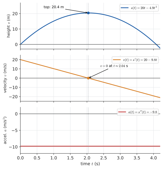
The second derivative has a geometric meaning too: it is the rate at which the slope changes, so it measures concavity. \(f'' > 0\) means slopes are increasing (the graph bends upwards, like a cup); \(f'' < 0\) means it bends downwards. That is the backbone of the second-derivative test in Chapter 18.
A pattern for the curious. Differentiate \(\sin x\) repeatedly: \(\cos x, -\sin x, -\cos x, \sin x, \dots\): period four. Differentiate \(x^4\): \(4x^3, 12x^2, 24x, 24, 0, 0, \dots\): a polynomial of degree \(n\) dies after \(n+1\) differentiations. Both facts are the seeds of Taylor series, previewed in Chapter 18.
|
Jerk and the smooth lift
Engineers care about the third derivative. A lift that switches instantly from zero to constant acceleration has infinite jerk at that moment, which you feel as a lurch. Lifts, trains, roller coasters, CNC machines and camera-motion paths in games are designed with bounded jerk (and sometimes bounded fourth derivative, whimsically called snap, followed by crackle and pop). |
Where else second derivatives turn up. A news report saying "inflation is still rising, but more slowly" is a statement about a second derivative: prices are increasing (\(P' > 0\)) and the rate of increase is falling (\(P'' < 0\)). In a physics engine, Newton’s second law \(F = m\ddot{x}\) is turned into code by computing acceleration from forces each frame and stepping velocity and position forward (Euler’s method, Chapter 19). And in optimisation the second derivative measures curvature, telling Newton’s method how big a step to take (Chapter 18).
17.9. When the derivative does not exist
17.9.1. The problem
Every rule so far assumed the limit in the definition exists. It doesn’t always. Understanding how it can fail sharpens what the derivative means, and the failures appear in practice: the ReLU activation in neural networks has a corner, and absolute-value loss functions have corners exactly at their minimum. So does UK income tax: tax owed is a continuous function of income, but its slope (your marginal rate) jumps from 20% to 40% at the higher-rate threshold (£50,270 in recent tax years). Just below it, an extra £100 of pay costs £20 in income tax; just above, £40. The graph has a corner there, and "the" derivative at the threshold does not exist.
17.9.2. Three ways to fail
A corner: \(f(x) = \lvert x \rvert\) at \(x = 0\). The difference quotient is \(\dfrac{\lvert h \rvert - 0}{h}\), which equals \(+1\) for \(h > 0\) and \(-1\) for \(h < 0\). The one-sided limits disagree (\(+1\) from the right, \(-1\) from the left), so the two-sided limit does not exist. Geometrically: secants from the right and secants from the left settle on two different lines. There is no single tangent.
A cusp: \(f(x) = x^{2/3}\) at \(x = 0\). The difference quotient is \(\dfrac{h^{2/3}}{h} = h^{-1/3}\), which tends to \(-\infty\) as \(h \to 0^-\) and to \(\infty\) (positive infinity) as \(h\) shrinks to 0 from the right. The graph comes into the origin vertically from both sides and turns back on itself.
A vertical tangent: \(f(x) = x^{1/3}\) at \(x = 0\). The difference quotient is \(\dfrac{h^{1/3}}{h} = h^{-2/3} \to +\infty\) from both sides. There is a tangent line (the \(y\)-axis), but its slope is infinite, and the derivative must be a finite number.
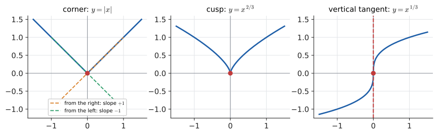
A fourth: discontinuity. If \(f\) jumps at \(a\), it cannot be differentiable there. In fact: Try it: Left and right slopes of |x|.
Proof (one line, and worth it): \(f(a+h) - f(a) = \dfrac{f(a+h) - f(a)}{h}\cdot h \to f'(a)\cdot 0 = 0\) as \(h \to 0\), so \(f(a+h) \to f(a)\). The converse is false: \(\lvert x \rvert\) is continuous everywhere but not differentiable at 0.
|
Continuous is not the same as smooth
"No breaks in the graph" (continuity) does not guarantee "a well-defined slope" (differentiability). When you differentiate a formula with the rules, you get an answer wherever the rules apply, and the rules can quietly hide the problem points: the power rule gives \(\frac{d}{dx}x^{1/3} = \tfrac13 x^{-2/3}\), which is undefined at 0. That undefined value is the formula telling you something. Check piecewise definitions, absolute values, and fractional powers at the points where pieces meet or the formula blows up. |
|
Continuous everywhere, differentiable nowhere
In 1872 Karl Weierstrass exhibited a function, \(\sum_{n=0}^{\infty} a^n\cos(b^n\pi x)\) with suitable \(a, b\), that is continuous everywhere but has a corner at every point. Mathematicians of the time called such functions "monsters". Today they’re everyday objects: the path of a Brownian particle, and the stock-price models built on it, are continuous but nowhere differentiable. Zoom into a smooth curve and it straightens out; zoom into these and they stay jagged at every scale, like a fractal. |
17.10. How computers compute derivatives
You have a function in code, not a formula on paper: a simulation, a rendering pipeline, a neural network with ten million parameters. You need its derivative. There are three approaches, and every working engineer should know which is which.
17.10.1. Numerical differentiation: just use a small \(h\)
The definition says the difference quotient approaches \(f'(x)\) as \(h \to 0\). So pick a small \(h\) and compute it. Two common formulas:
The central difference uses a secant that straddles \(x\) symmetrically. Draw it on a parabola and you’ll see why it’s better: the errors on the two sides cancel. In fact for a quadratic the central difference is exact for any \(h\).
How big is the error? Taylor polynomials (Chapter 18) tell us \(f(x+h) = f(x) + hf'(x) + \tfrac{h^2}{2}f''(x) + \tfrac{h^3}{6}f'''(x) + \cdots\). Substituting:
This truncation error says: make \(h\) smaller, get a better answer. Shrinking \(h\) by 10 cuts the forward error by 10 and the central error by 100.
But computers don’t do real arithmetic; they do floating point (Chapter 1), with about 16 significant digits (\(\varepsilon \approx 2.2\times 10^{-16}\)). When \(h\) is tiny, \(f(x+h)\) and \(f(x)\) agree in most of their digits, and subtracting them (catastrophic cancellation) leaves only a few meaningful digits. Each value carries a rounding error of about \(\varepsilon\lvert f \rvert\), and dividing by \(h\) amplifies it to about \(\varepsilon\lvert f \rvert / h\). This rounding error grows as \(h\) shrinks.
Let’s measure both. Differentiate \(\sin\) at \(x = 1\); the exact answer is \(\cos 1\).
import math

def forward_diff(f, x, h):
    return (f(x + h) - f(x)) / h

def central_diff(f, x, h):
    return (f(x + h) - f(x - h)) / (2 * h)

exact = math.cos(1.0)
print(f"{'h':>8} {'forward error':>15} {'central error':>15}")
for k in range(1, 13, 1):
    h = 10.0 ** -k
    ef = abs(forward_diff(math.sin, 1.0, h) - exact)
    ec = abs(central_diff(math.sin, 1.0, h) - exact)
    print(f"{h:8.0e} {ef:15.3e} {ec:15.3e}")
h forward error central error 1e-01 4.294e-02 9.001e-04 1e-02 4.216e-03 9.005e-06 1e-03 4.208e-04 9.005e-08 1e-04 4.207e-05 9.004e-10 1e-05 4.207e-06 1.114e-11 1e-06 4.207e-07 2.772e-11 1e-07 4.183e-08 1.943e-10 1e-08 1.407e-08 2.970e-09 1e-09 5.254e-08 2.970e-09 1e-10 5.848e-08 5.848e-08 1e-11 1.169e-06 1.169e-06 1e-12 4.324e-05 1.227e-05
The theory predicts the top of the table exactly: forward error \(\approx \tfrac{h}{2}\lvert\sin 1\rvert = 0.42h\), central error \(\approx \tfrac{h^2}{6}\cos 1 = 0.090h^2\). Then the trend reverses. The forward difference is best around \(h \approx 10^{-8} \approx \sqrt{\varepsilon}\), with about 8 correct digits; the central difference is best around \(h \approx 10^{-5} \approx \varepsilon^{1/3}\), with about 11. Make \(h\) smaller than that and the answer gets worse.
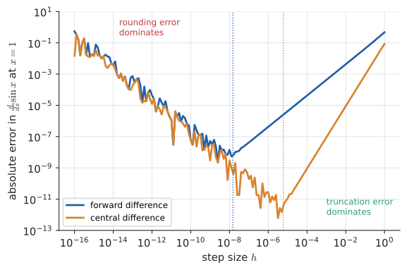
|
Smaller is not always better
"Take the limit as \(h \to 0\)" is a mathematical instruction, not a numerical one. In floating point, \(h = 10^{-15}\) gives a derivative with essentially no correct digits, and \(h = 10^{-17}\) gives zero, because \(1 + 10^{-17}\) rounds to exactly \(1\). Rules of thumb: forward difference \(h \approx 10^{-8}\cdot\max(1, \lvert x \rvert)\); central difference \(h \approx 10^{-5}\cdot\max(1, \lvert x \rvert)\). And numerical derivatives of noisy data (sensor readings) amplify the noise; smooth first. |
|
Finding the sweet spot
A slider sets \(\log_{10} h\) from \(-16\) to 0 and plots forward and central difference errors for a function you choose (\(\sin\), \(e^x\), \(x^3\), \(\sqrt{x}\) near 0). Find the best \(h\) for each. Then switch to 32-bit floats and watch the sweet spot move to much larger \(h\). |
17.10.2. Automatic differentiation: exact derivatives without formulas
Numerical differentiation is approximate and fragile. Symbolic differentiation (applying the rules to a formula tree, as SymPy does) is exact but needs a formula and can produce enormous expressions. There is a third way, and it powers essentially all modern machine learning: automatic differentiation (AD). It applies the rules of this chapter, not to formulas, but to the actual numbers flowing through your program. Try it: Dual numbers, node by node.
The forward-mode version rests on a small algebraic trick. Invent a number \(\epsilon\) with \(\epsilon \neq 0\) but \(\epsilon^2 = 0\) (like \(i^2 = -1\) in Chapter 15, it’s an extension of the number system defined by a rule). Numbers of the form \(a + b\epsilon\) are called dual numbers. Multiply two:
The \(\epsilon\) part is the product rule: if \(b\) and \(d\) are the derivatives of two quantities \(a\) and \(c\), then \(ad + bc\) is the derivative of their product. More generally, for any polynomial \(f\), expanding \(f(x + \epsilon)\) gives \(f(x) + f'(x)\epsilon\) exactly, because every \(\epsilon^2\) and higher term vanishes. Evaluate your function on \(x + 1\epsilon\) and the derivative falls out in the \(\epsilon\) slot, exact to floating-point precision, with no \(h\) to choose.
import math

class Dual:
    """A number a + b*eps with eps**2 == 0. b carries the derivative."""
    def __init__(self, val, der=0.0):
        self.val, self.der = val, der

    def __add__(self, other):
        other = other if isinstance(other, Dual) else Dual(other)
        return Dual(self.val + other.val, self.der + other.der)
    __radd__ = __add__

    def __sub__(self, other):
        other = other if isinstance(other, Dual) else Dual(other)
        return Dual(self.val - other.val, self.der - other.der)

    def __mul__(self, other):
        other = other if isinstance(other, Dual) else Dual(other)
        # product rule lives here
        return Dual(self.val * other.val,
                    self.der * other.val + self.val * other.der)
    __rmul__ = __mul__

    def __truediv__(self, other):
        other = other if isinstance(other, Dual) else Dual(other)
        # quotient rule lives here
        return Dual(self.val / other.val,
                    (self.der * other.val - self.val * other.der) / other.val ** 2)

def sin(x):
    # chain rule: d/dx sin(u) = cos(u) * u'
    return Dual(math.sin(x.val), math.cos(x.val) * x.der)

def exp(x):
    return Dual(math.exp(x.val), math.exp(x.val) * x.der)

def derivative(f, x):
    return f(Dual(x, 1.0)).der

f = lambda x: x * x * x + 2 * x          # f'(x) = 3x^2 + 2
g = lambda x: sin(x * x)                  # g'(x) = 2x cos(x^2)
h = lambda x: exp(2 * x) / (1 + x * x)    # quotient + chain

print(derivative(f, 2.0))
print(derivative(g, 1.5), 2 * 1.5 * math.cos(1.5 ** 2))
x = 0.5
exact_h = (2 * math.exp(2*x) * (1 + x*x) - math.exp(2*x) * 2*x) / (1 + x*x)**2
print(derivative(h, 0.5), exact_h)
14.0 -1.8845208681682175 -1.8845208681682175 2.609550555320683 2.609550555320683
Look at what each method of the class contains: the sum rule, the product rule, the quotient rule, and (in sin and exp) the chain rule. The rules of this chapter are the whole implementation. The derivatives agree with the hand-derived formulas to every printed digit.
17.10.3. Backpropagation is the chain rule
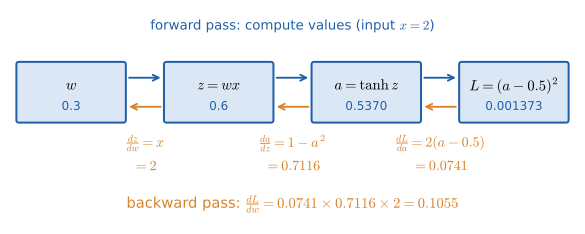
Forward mode pushes one derivative through the program alongside the values. That costs one pass per input variable. A neural network has millions of inputs (its weights) and one output (the loss), so forward mode would need millions of passes. Reverse mode turns it around: run the program forward once, recording intermediate values, then walk backwards multiplying local derivatives via the chain rule. One backward pass gives the derivative of the output with respect to every input. In machine learning, reverse-mode AD is called backpropagation. Try it: Backpropagate the one-weight network.
Here is a one-weight "network": input \(x\), weight \(w\), prediction \(a = \tanh(wx)\), loss \(L = (a - \text{target})^2\). As a chain: \(w \to z = wx \to a = \tanh z \to L\). The chain rule says
using \(\frac{d}{dz}\tanh z = 1 - \tanh^2 z\).
import math

def loss(w, x=2.0, target=0.5):
    z = w * x                 # stage 1
    a = math.tanh(z)          # stage 2
    return (a - target) ** 2  # stage 3

def grad_loss(w, x=2.0, target=0.5):
    # forward pass: remember intermediate values
    z = w * x
    a = math.tanh(z)
    L = (a - target) ** 2
    # backward pass: multiply local derivatives, last stage first
    dL_da = 2 * (a - target)
    da_dz = 1 - a ** 2        # derivative of tanh
    dz_dw = x
    return L, dL_da * da_dz * dz_dw

w = 0.3
L, g = grad_loss(w)
numeric = (loss(w + 1e-6) - loss(w - 1e-6)) / 2e-6
print(f"loss = {L:.6f}")
print(f"chain-rule gradient = {g:.6f}")
print(f"central-difference  = {numeric:.6f}")
loss = 0.001373 chain-rule gradient = 0.105455 central-difference = 0.105455
The central difference is used here the way practitioners use it: as a gradient check, an independent test that the hand-written backward pass is right. A real network has millions of weights and many layers, so the chain has many links and branches, but every step of backpropagation is this: a local derivative, multiplied into the running product, from the output back towards the inputs. Gradient descent (Chapter 18, Chapter 20, Chapter 33) then nudges each weight downhill.
|
Why it took until the 2010s
Reverse-mode automatic differentiation was described by Seppo Linnainmaa in his 1970 master’s thesis, and backpropagation for neural networks was popularised by Rumelhart, Hinton and Williams in 1986. The mathematics, the chain rule, is from Leibniz’s notebooks of the 1670s. What changed in the 2010s was data and GPUs; the calculus was already three centuries old. |
|
Build a computation graph
Drag nodes (\(+\), \(\times\), \(\sin\), \(\exp\), \(x^2\)) onto a canvas to build an expression graph. Press "forward" to watch values flow from inputs to output; press "backward" to watch local derivatives multiply their way back from the output, with each edge labelled by its local derivative. Compare the result with forward-mode dual numbers and with a finite difference. Try it: Build a computation graph |
17.11. Chapter exercises
-
(Recognition) Which of these is the definition of \(f'(2)\)? (a) \(\dfrac{f(2+h) - f(2)}{h}\); (b) \(\lim_{h\to0}\dfrac{f(2+h) - f(2)}{h}\); (c) \(\lim_{h\to0}\dfrac{f(h) - f(2)}{h}\).
-
(Recognition) For each, name the rule(s) you would use first: \(e^x\cos x\); \(\cos(e^x)\); \(\dfrac{e^x}{\cos x}\); \(e^x + \cos x\).
-
(Application) Differentiate: (a) \(x^3 e^{2x}\); (b) \(\ln(\cos x)\); (c) \(\dfrac{\sin x}{1 + \cos x}\); (d) \(e^{\sin 3x}\).
-
(Application) A particle moves with \(s(t) = t^3 - 9t^2 + 24t\) metres. When is it momentarily at rest? What is its acceleration at those times?
-
(Problem solving) Find the equation of the tangent line to \(y = x\ln x\) at \(x = e\).
-
(Problem solving) For what value of \(k\) is the piecewise function \(f(x) = x^2\) for \(x \le 1\), \(f(x) = kx - 1\) for \(x > 1\) both continuous and differentiable at \(x = 1\)?
-
(Problem solving, CS) Extend the
Dualclass with acosfunction and apowmethod for a constant integer exponent. Test on \(\cos(x^3)\) at \(x = 1\).
Answers
-
(b). Option (a) has no limit, so it is a secant slope; (c) uses the wrong numerator.
-
Product rule; chain rule; quotient rule; sum rule.
-
(a) Product + chain: \(3x^2 e^{2x} + x^3\cdot 2e^{2x} = x^2 e^{2x}(3 + 2x)\). (b) Chain: \(\dfrac{1}{\cos x}\cdot(-\sin x) = -\tan x\). (c) Quotient: \(\dfrac{\cos x(1 + \cos x) - \sin x(-\sin x)}{(1 + \cos x)^2} = \dfrac{\cos x + \cos^2 x + \sin^2 x}{(1+\cos x)^2} = \dfrac{1 + \cos x}{(1 + \cos x)^2} = \dfrac{1}{1 + \cos x}\). (d) Chain, two layers: \(e^{\sin 3x}\cdot\cos 3x\cdot 3 = 3\cos(3x)\,e^{\sin 3x}\).
-
\(v = 3t^2 - 18t + 24 = 3(t^2 - 6t + 8) = 3(t-2)(t-4)\), so at rest at \(t = 2\) and \(t = 4\) s. \(a = 6t - 18\): \(a(2) = -6\) m/s² (slowing to a stop then reversing), \(a(4) = 6\) m/s².
-
\(y' = 1\cdot\ln x + x\cdot\tfrac1x = \ln x + 1\). At \(x = e\): \(y = e\ln e = e\), slope \(= 1 + 1 = 2\). Tangent: \(y - e = 2(x - e)\), i.e. \(y = 2x - e\).
-
Continuity at 1: \(1^2 = k\cdot 1 - 1\), so \(k = 2\). Differentiability: left derivative \(2x = 2\) at \(x=1\); right derivative \(k = 2\). They match, so \(k = 2\) gives both.
-
One possible solution:
def cos(x):
    return Dual(math.cos(x.val), -math.sin(x.val) * x.der)

def _pow(self, n):           # n a plain int
    return Dual(self.val ** n, n * self.val ** (n - 1) * self.der)
Dual.__pow__ = _pow

print(derivative(lambda x: cos(x ** 3), 1.0))   # -2.5244129544236893
print(-3 * math.sin(1.0))                         # same: -3 x^2 sin(x^3) at 1
17.12. Interactive tools
Browser tools on the companion website that go with this chapter. Each example link in the chapter opens one of them with that example already set up.
17.13. Mastery check
-
Using the definition, find \(f'(x)\) for \(f(x) = 3x^2 - x\).
-
Differentiate \(y = x^3 e^x\).
-
Differentiate \(y = \ln(x^2 + 1)\).
-
Differentiate \(y = \dfrac{\sin x}{x}\).
-
Find \(dy/dx\) at \((1, 2)\) on the curve \(x^2 + xy + y^2 = 7\).
-
Where is \(f(x) = \lvert x - 2 \rvert\) not differentiable, and why?
-
A particle has position \(s(t) = t^3 - 6t^2 + 9t\). Find its velocity and acceleration at \(t = 2\).
-
You estimate \(\frac{d}{dx}e^x\) at \(x = 0\) with a forward difference and \(h = 10^{-3}\). Roughly how large is the error, and how would you reduce it?
Decision rule: All correct without hesitation → move on to Chapter 18. Stuck on 1 → reread Section 17.4. Stuck on 2–4 → reread Section 17.5 and Section 17.6 and do their exercises. Stuck on 5 → Section 17.7. Stuck on 6 → Section 17.9. Stuck on 8 → Section 17.10.
Mastery check answers
-
\(\dfrac{3(x+h)^2 - (x+h) - 3x^2 + x}{h} = \dfrac{6xh + 3h^2 - h}{h} = 6x + 3h - 1 \to 6x - 1\).
-
Product rule: \(3x^2 e^x + x^3 e^x = x^2(x + 3)e^x\).
-
Chain rule: \(\dfrac{1}{x^2 + 1}\cdot 2x = \dfrac{2x}{x^2 + 1}\).
-
Quotient rule: \(\dfrac{x\cos x - \sin x}{x^2}\).
-
Check: \(1 + 2 + 4 = 7\). Differentiate: \(2x + (y + x\,y') + 2y\,y' = 0\), so \(y'(x + 2y) = -(2x + y)\), \(y' = -\dfrac{2x + y}{x + 2y}\). At \((1,2)\): \(-\dfrac{4}{5}\).
-
At \(x = 2\) only. It has a corner there: the left derivative is \(-1\) and the right derivative is \(+1\), so the limit of the difference quotient does not exist. It is still continuous there.
-
\(v = 3t^2 - 12t + 9\), so \(v(2) = 12 - 24 + 9 = -3\) m/s (moving backwards). \(a = 6t - 12\), so \(a(2) = 0\).
-
Truncation error \(\approx \tfrac{h}{2}f''(0) = \tfrac{10^{-3}}{2}\cdot 1 = 5\times10^{-4}\); indeed \((e^{0.001} - 1)/0.001 = 1.0005002\). Reduce it by switching to a central difference (error \(\approx h^2/6 \approx 1.7\times 10^{-7}\) at the same \(h\)), or by decreasing \(h\) towards \(10^{-8}\) but no further (rounding error takes over), or by using automatic differentiation, which is exact.