Volume 2: Continuous Mathematics · Part IX: Numerical Mathematics
Chapter 32. Numerical Mathematics: How Computers Actually Compute
Every earlier chapter quietly assumed that numbers are exact. Inside a computer they are not. This chapter shows how real numbers are actually stored, where the errors come from, how they grow or stay tame, and how to choose algorithms that give answers you can trust. We revisit root finding, derivatives, integrals, linear systems, differential equations and interpolation, this time as a numerical analyst sees them: understand the method, calculate a few steps by hand, implement it, and then experiment until it breaks.
32.1. The problem: the machine is not doing real-number arithmetic
Open a Python prompt and type:
print(0.1 + 0.2)
print(0.1 + 0.2 == 0.3)
0.30000000000000004 False
This is not a Python bug. The same thing happens in C, Java, JavaScript, Excel and on your phone’s calculator app if it is honest. The computer cannot store 0.1 exactly, it cannot store 0.2 exactly, and the sum of the two stored values is not the stored value of 0.3.
Most of the time the discrepancy is in the sixteenth significant digit and nobody cares. But errors can grow. Three real incidents give the flavour:
-
In 1991 a Patriot missile battery in Dhahran failed to intercept an incoming Scud. Its clock counted tenths of a second in a 24-bit fixed-point register; 0.1 has no finite binary expansion, so every tick lost about \(9.5\times 10^{-8}\) seconds. After 100 hours of continuous running the accumulated drift was about 0.34 s, enough for the target to be some 500 m from where the system looked.
-
In 1996 the first Ariane 5 rocket self-destructed 37 seconds after launch when a 64-bit floating-point velocity value was converted to a 16-bit integer and overflowed.
-
In 1982 the Vancouver Stock Exchange started a new index at 1000. It was recomputed thousands of times a day and truncated (chopped) to three decimal places each time rather than rounded. Twenty-two months later it stood near 525; recomputed correctly it should have been about 1099.
None of these was a failure of the mathematics on paper. Each was a failure to understand how the mathematics behaves once it is executed by a finite machine. That understanding is the subject of numerical mathematics (or numerical analysis): the study of algorithms that compute approximate answers to continuous problems, together with rigorous statements about how good those approximations are.
|
Numerical analysis
Numerical analysis is the branch of mathematics that designs and analyses algorithms for approximating answers to problems (roots, integrals, derivatives, solutions of equations) when exact symbolic answers are unavailable, too expensive, or meaningless because the data are themselves approximate. Its two central questions are how fast does the method approach the answer? and how much error does it introduce? |
32.2. Floating point: how real numbers are stored
32.2.1. The problem
A real number such as \(\pi\) has infinitely many digits. Memory is finite. Something has to give. The question is what to give up so that the arithmetic is fast, predictable, and good enough for numbers as different as the mass of an electron (\(9.1\times10^{-31}\) kg) and the number of atoms in the observable universe (about \(10^{80}\)).
32.2.2. Intuition: scientific notation with a fixed budget of digits
You already know the answer from science class. Instead of writing 0.000000000000000000000000000000911, you write \(9.11\times10^{-31}\): a handful of significant digits and an exponent that says where the decimal point goes. The decimal point "floats" to wherever it is needed; hence floating point.
A computer does the same in base 2, with a fixed budget: in the standard 64-bit "double precision" format, 53 significant binary digits (bits) and an 11-bit exponent. Fixing the number of significant digits rather than the number of decimal places has a crucial consequence: the relative accuracy is the same everywhere, but the absolute spacing between representable numbers grows with their size. Between 1 and 2 there are \(2^{52}\) evenly spaced doubles; between 1024 and 2048 there are also \(2^{52}\), spread over a range 1024 times wider.
|
Significand, exponent, floating point
A floating-point number has the form \(\pm\, m\times\beta^{e}\), where \(\beta\) is the base (2 in hardware), \(m\) is the significand (also called the mantissa) holding a fixed number of significant digits, and \(e\) is the integer exponent. In base 2 the significand of a nonzero number can always be scaled so that it looks like \(1.f_1f_2f_3\ldots\) in binary; this is the normalised form, and the bits \(f_1f_2\ldots\) are the fraction. |
32.2.3. Why it works: the IEEE 754 double
Since 1985 essentially every processor has implemented the IEEE 754 standard. A double occupies 64 bits split into three fields.
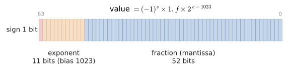
For an ordinary ("normal") number the value is
where \(s\) is the sign bit, \(f\) is the 52-bit fraction read as an integer, and \(E\) is the 11-bit exponent field read as an integer between 1 and 2046. The leading 1 of the significand is not stored (it is always 1 for a normal number), which buys an extra bit for free: 52 stored bits give 53 bits of precision. The bias of 1023 lets the stored field be unsigned while the true exponent \(E-1023\) runs from \(-1022\) to \(+1023\).
The two leftover exponent patterns are reserved:
-
\(E=2047\) (all ones) encodes infinity (fraction zero) and NaN, "not a number" (fraction nonzero), the result of operations such as \(0/0\) or \(\infty-\infty\).
-
\(E=0\) (all zeros) encodes zero (there are two, \(+0\) and \(-0\)) and the subnormal numbers, which drop the hidden leading 1 to fill the gap between zero and the smallest normal number.
|
Range, overflow, underflow
The largest finite double is about \(1.80\times10^{308}\); the smallest positive normal double is about \(2.23\times10^{-308}\); the smallest positive subnormal is about \(4.9\times10^{-324}\). A result too large to represent overflows to \(\pm\infty\). A result too small underflows, first gradually through the subnormals (losing precision) and finally to zero. |
32.2.4. Worked example: what is actually stored for 0.1?
Let us convert 0.1 to binary by hand. To find binary digits after the point, repeatedly multiply by 2 and peel off the integer part:
So \(0.1_{10} = 0.0\overline{0011}_2 = 0.000110011001100\ldots_2\). Like \(1/3=0.333\ldots\) in decimal, it never terminates. The reason is that \(0.1 = 1/10\) and 10 has the prime factor 5, which is not a factor of the base 2. Only fractions whose denominators are powers of 2 terminate in binary.
Normalise by moving the point four places right:
-
Sign: positive, so \(s=0\).
-
Exponent: true exponent \(-4\), so the stored field is \(E=-4+1023=1019 = 01111111011_2\).
-
Fraction: the 52 bits after the leading 1 are \(1001\,1001\ldots1001\) followed by \(1010\); the infinite tail \(1001\ldots\) beyond bit 52 starts with a 1, so the last kept group \(1001\) rounds up to \(1010\).
In hexadecimal the whole 64-bit word is 3FB999999999999A; the final A (rather than 9) is the round-up. Because we rounded up, the stored value is slightly larger than 0.1. Python can show its exact decimal value:
from decimal import Decimal
import struct

print(Decimal(0.1))                      # exact value of the stored double
print(struct.pack('>d', 0.1).hex())      # its 64 raw bits in hex
0.1000000000000000055511151231257827021181583404541015625 3fb999999999999a
Now the puzzle of the opening dissolves. The doubles nearest to 0.1, 0.2 and 0.3 are
Their exact sum is \(0.3000000000000000166533\ldots\); rounding that to the nearest double gives \(0.3000000000000000444089\ldots\), which is the double just above \(\mathrm{fl}(0.3)\). Python prints the shortest decimal string that uniquely identifies it: 0.30000000000000004.
32.2.5. Vocabulary: machine epsilon and the ulp
|
Machine epsilon and unit roundoff
Machine epsilon \(\varepsilon_{\text{mach}}\) is the gap between 1 and the next larger floating-point number. For doubles \(\varepsilon_{\text{mach}} = 2^{-52}\approx 2.22\times10^{-16}\). The unit roundoff \(u=\varepsilon_{\text{mach}}/2 = 2^{-53}\approx1.11\times10^{-16}\) is the largest relative error committed by rounding a real number (in range) to the nearest double. "Doubles carry about 16 significant decimal digits" is shorthand for \(-\log_{10}u\approx 15.95\). |
|
Ulp
An ulp (unit in the last place) of a floating-point number \(x\) is the gap between \(x\) and the next representable number of larger magnitude. \(\mathrm{ulp}(1)=2^{-52}\); \(\mathrm{ulp}(10^{16}) = 2\). Errors are often quoted in ulps: "correctly rounded" means within half an ulp. |
The single most useful model of floating-point arithmetic follows from these definitions. IEEE 754 requires that the basic operations \(+,-,\times,\div\) and \(\sqrt{\ }\) be correctly rounded: the result is the exact answer rounded to the nearest double. So for any of these operations, written \(\circ\),
Read it aloud: each individual operation is wrong by a relative amount no larger than about \(10^{-16}\). All the drama in this chapter comes not from a single operation but from how such tiny relative errors are amplified by what we do next.
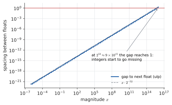
The diagram shows the spacing between doubles as a function of their size. It is a staircase (constant within each power-of-two band, then doubling) that looks like a straight line on log-log axes. At \(2^{53}=9\,007\,199\,254\,740\,992\) the gap reaches 1, so \(2^{53}+1\) cannot be stored: float(2**53 + 1) returns 9007199254740992.0. This is why JavaScript, whose only number type is the double, defines Number.MAX_SAFE_INTEGER as \(2^{53}-1\).
|
Never test floats for exact equality
A purely relative tolerance fails near zero (nothing is relatively close to 0 except 0); a purely absolute one fails for large numbers (\(10^{20}\) and \(10^{20}+1\) are "far apart" in absolute terms but identical as doubles). Note also that |
|
The man who designed your arithmetic
Before 1985 every manufacturer had its own floating-point format, with its own rounding quirks; porting numerical code was a nightmare, and some machines could produce \(x\ne y\) yet \(x-y=0\). William Kahan of Berkeley led the design of IEEE 754 (working closely with Intel on the 8087 coprocessor) and received the 1989 Turing Award for it. Subnormal numbers, his idea, guarantee that \(x-y=0\) if and only if \(x=y\). |
|
Float explorer
Type any decimal number and see its 64 bits coloured by field, its exact stored value, the neighbouring doubles on either side, and its ulp. Drag a slider through magnitudes from \(10^{-320}\) to \(10^{308}\) and watch the spacing change, the subnormal region appear, and the value finally overflow to infinity. |
32.2.6. Where you’d use this
-
Maps and GPS. A latitude of 51.5° stored as a 32-bit float can only take values about \(3.8\times10^{-6}\) degrees apart, which on the ground is about 0.42 m. Fine for a running app; useless for a surveyor or a self-driving car, which store coordinates as doubles (gap about a nanometre). The same arithmetic explains why a flight simulator that stores the plane’s position in metres from the centre of the Earth (about \(6.4\times10^{6}\) m) in float32 can only move it in 0.5 m jumps.
-
Money and spreadsheets. A program that adds 0.1 ten times gets
0.9999999999999999, so a test for equality with 1 fails. Accounting systems avoid this by counting in integer pennies; when you see a bank statement off by a penny, a binary-float rounding is a prime suspect. -
Science: astronomers and physicists who need more than 16 digits (pulsar timing, long-baseline interferometry) use double-double or quadruple-precision arithmetic, because the ulp of a double is too coarse for the quantities they measure.
32.3. Rounding error and catastrophic cancellation
32.3.1. The problem
Solve \(x^2 + 10^8x + 1 = 0\). The quadratic formula from Chapter 8 gives Try it: Cancellation and the stable rewrite.
The two roots are about \(-10^8\) and about \(-10^{-8}\) (their product is \(c/a=1\)). In double precision:
import math
a, b, c = 1.0, 1e8, 1.0
d = math.sqrt(b*b - 4*a*c)
print((-b + d) / (2*a))      # the small root, computed naively
print((-b - d) / (2*a))      # the large root
-7.450580596923828e-09 -100000000.0
The large root is fine. The small root should be \(-1.0000000000000000\ldots\times10^{-8}\); we got \(-7.45\times10^{-9}\), wrong in the first significant digit. A 25% error from a calculation in which every single operation was accurate to 16 digits. What happened?
32.3.2. Intuition: subtraction of nearly equal numbers
|
Absolute and relative error
If \(\hat x\) approximates \(x\), the absolute error is \(|\hat x - x|\) and the relative error is \(|\hat x - x|/|x|\) (for \(x\ne0\)). Relative error \(10^{-k}\) means roughly \(k\) correct significant digits. Floating point controls relative error; that is its whole design. |
Here \(b=10^8\) and \(\sqrt{b^2-4}\) are equal in their first 16 digits:
The computed square root carries a relative error up to \(u\), i.e. an absolute error up to about \(10^8\times10^{-16}=10^{-8}\). Subtraction \(-b+d\) is itself performed exactly (the two numbers are so close that the difference is representable), but it removes the 16 digits they share and leaves only what was in the "noise" region. The absolute error of about \(10^{-8}\) is now attached to a result of size \(2\times10^{-8}\): relative error of order 1. This is catastrophic cancellation.
The key insight: subtraction does not create error; it exposes error that was already present in its inputs. If the inputs were exact, the difference would be exact.
32.3.3. The method: rewrite to avoid the subtraction
The cure is algebra. Rationalise the numerator (multiply top and bottom by the conjugate):
Now the denominator adds two numbers of the same sign: no cancellation. With our numbers, \(2c/(-b-d) = 2/(-2\times10^8) = -1.0\times10^{-8}\) to full precision. Equivalently, use the product of roots: \(x_{\text{small}} = c/(a\,x_{\text{large}})\).
Input: a formula to be evaluated in floating point.
Steps:
-
Look for subtractions \(A-B\) (or additions of opposite signs) where \(A\) and \(B\) can be nearly equal for the inputs you care about.
-
Check whether \(A\) and \(B\) are themselves the result of rounding (a square root, a cosine, a measured value). If they are exact, the subtraction is harmless.
-
If they are inexact, rewrite algebraically so the cancellation happens symbolically, not numerically: multiply by a conjugate, use a trigonometric identity, use a Taylor series for small arguments, or use a library function designed for the job.
-
Test the rewritten formula against a high-precision reference (Python’s
decimalorfractions) at extreme inputs.
Output: an algebraically equivalent formula whose floating-point evaluation keeps its relative accuracy.
Some standard rewrites:
| Dangerous form | Safe form | Why |
|---|---|---|
\(1-\cos x\) for small \(x\) |
\(2\sin^2(x/2)\) |
identity; no subtraction |
\(\sqrt{x+1}-\sqrt{x}\) for large \(x\) |
\(1/(\sqrt{x+1}+\sqrt{x})\) |
conjugate |
\(\ln(1+x)\) for small \(x\) |
|
\(1+x\) would round away \(x\) |
\(e^x-1\) for small \(x\) |
|
same reason |
\(\sqrt{x^2+y^2}\) |
|
\(x^2\) may overflow |
For \(x=10^{-8}\), 1 - math.cos(x) returns exactly 0.0 (because \(\cos(10^{-8}) = 1 - 5\times10^{-17}\) rounds to 1), while 2*math.sin(x/2)**2 returns 5.0000000000000005e-17, correct to 16 digits.
32.3.4. Overflow and underflow in practice
The other two floating-point hazards are about range, not precision.
Overflow. Computing \(\sqrt{x^2+y^2}\) for \(x=10^{200}\) overflows at \(x^2\) even though the answer, about \(10^{200}\), is perfectly representable. math.hypot rescales internally.
Underflow. Multiply the probabilities of 1000 independent events, each 0.01, and the true answer \(10^{-2000}\) underflows to 0. Every probabilistic model that multiplies many likelihoods therefore works with logarithms: \(\log\prod p_i = \sum\log p_i\) turns a product that underflows into a sum that is perfectly well behaved (Chapter 12).
|
Cancellation in disguise
The textbook variance formula \(\frac1n\sum x_i^2 - \bar x^{\,2}\) (Chapter 31) subtracts two large, nearly equal numbers when the data have a large mean and small spread (timestamps in nanoseconds, say). It can even return a negative variance. Use the two-pass formula \(\frac1n\sum(x_i-\bar x)^2\), or Welford’s one-pass update, instead. |
32.4. Conditioning versus stability
32.4.1. The problem
When a computed answer is bad, whose fault is it? Sometimes the problem is so sensitive that no algorithm could do better; sometimes a perfectly reasonable problem was solved with a bad algorithm. Numerical analysts keep these two ideas strictly separate, and you should too.
32.4.2. Conditioning: a property of the problem
Consider the system Try it: Nudge the right-hand side; Feel κ ≈ 4 × 10⁴.
Subtracting the first equation from the second gives \(0.0001\,y=0.0001\), so \(y=1\) and \(x=1\). Now change the right-hand side of the second equation by one part in 20,000, from \(2.0001\) to \(2.0002\). Then \(0.0001\,y = 0.0002\), so \(y=2\) and \(x=0\). A change in the fifth significant digit of the data moved the answer from \((1,1)\) to \((0,2)\).
Geometrically, the two equations are lines that are almost parallel (Chapter 6). Nudge either one and their intersection slides a long way along them. No algorithm, however careful, can fix that: if the data carry an uncertainty of \(10^{-4}\), the answer is uncertain in its first digit.
|
Condition number
The condition number \(\kappa\) of a problem measures how much relative changes in the input are amplified in the output:
\[\frac{\text{relative change in output}}{\text{relative change in input}} \approx \kappa .\]
For a differentiable function of one variable, \(\kappa(x) = \left|\dfrac{x\,f'(x)}{f(x)}\right|\). For a linear system \(A\mathbf x=\mathbf b\), \(\kappa(A)=\|A\|\,\|A^{-1}\|\) (Chapter 27). A problem is well-conditioned if \(\kappa\) is modest and ill-conditioned if it is large. For the matrix above, \(\kappa\approx 4\times10^{4}\). |
Rule of thumb: you can lose about \(\log_{10}\kappa\) significant digits. With 16 digits available and \(\kappa=4\times10^4\), expect about 11 or 12 good digits from any decent solver, if the data themselves are exact.
The function \(f(x)=x-1\) near \(x=1\) is a one-variable example: \(\kappa = |x\cdot1/(x-1)|\), which blows up as \(x\to1\). That is catastrophic cancellation seen through the lens of conditioning: subtracting nearly equal numbers is an ill-conditioned operation.
32.4.3. Stability: a property of the algorithm
An algorithm is stable if it does not add much error beyond what the conditioning of the problem forces. The gold standard is backward stability: the computed answer is the exact answer to a slightly perturbed problem (perturbed by a few multiples of \(u\)). Then
This one line is the most important idea in numerical analysis. It splits every error into "the problem’s sensitivity" times "the algorithm’s sloppiness".
32.4.4. Worked example: one problem, a stable and an unstable algorithm
Define \(I_n = \int_0^1 x^n e^{x-1}\,dx\) for \(n=0,1,2,\ldots\). Integration by parts (Chapter 19) with \(u=x^n\), \(dv=e^{x-1}dx\) gives a recurrence: Try it: Forwards versus backwards recurrence.
Every \(I_n\) is positive (the integrand is positive) and they decrease (\(x^n\) shrinks on \(\lbrack 0,1\rbrack\)). Run the recurrence forwards in Python:
import math
I = 1 - 1/math.e                 # I_0
for n in range(1, 21):
    I = 1 - n * I
    if n in (5, 10, 15, 17, 18, 19, 20):
        print(n, I)
5 0.14553294057308008 10 0.0838770700582927 15 0.059033793641901866 17 0.05719187059730757 18 -0.029453670751536265 19 1.559619744279189 20 -30.19239488558378
A negative value at \(n=18\), then nonsense. Why? \(I_0\) is stored with error \(\delta\approx10^{-17}\). Each step multiplies the inherited error by \(-n\), so after 20 steps it has been multiplied by \(20!\approx2.4\times10^{18}\). The algorithm is wildly unstable, even though the problem (compute \(I_{20}\)) is perfectly well-conditioned.
Now run the same recurrence backwards: \(I_{n-1} = (1-I_n)/n\). Each step divides the error by \(n\). Start at \(n=40\) with the crude guess \(I_{40}=0\) (true value about 0.024, so the starting error is about 0.024):
J = 0.0                          # crude guess for I_40
for n in range(40, 20, -1):
    J = (1 - J) / n              # gives I_{n-1}
print(J)                         # I_20
0.045544884075818054
The starting error has been divided by \(40\cdot39\cdots21\approx 3.4\times10^{29}\); the answer is correct to all 16 digits. Same mathematics, same recurrence, opposite direction, opposite fate.
|
Ill-conditioned or unstable?
If a result is bad, first ask whether the problem is ill-conditioned (then improve the data, reformulate the question, or accept the uncertainty) or the algorithm unstable (then change the algorithm). Running in higher precision helps both, but only postpones the problem in the unstable case: with the forward recurrence above, quadruple precision merely moves the collapse from \(n=18\) to about \(n=30\). |
32.4.5. Where you’d use this
-
Navigation: GPS geometry. A GPS receiver solves for its position from distances to several satellites. If the satellites in view are bunched together in one part of the sky, the equations are like the nearly parallel lines above: ill-conditioned, so a few metres of timing noise becomes tens of metres of position error. Receivers report this amplification as the dilution of precision (DOP), a condition number with a friendlier name; surveyors schedule work for times when the satellites are well spread out.
-
Engineering and science: weather forecasting is famously ill-conditioned (the "butterfly effect"): tiny errors in today’s measurements grow until forecasts beyond about two weeks carry no skill, whatever the algorithm. Forecasters respond by running ensembles of slightly perturbed forecasts and reporting the spread, an honest answer to an ill-conditioned problem.
-
Computing: before blaming a library for a bad least-squares fit, check the condition number of the data matrix (
numpy.linalg.cond); near-duplicate input features (a price in pounds and the same price in dollars) make it huge.
32.5. Root finding compared
32.5.1. The problem
Solve \(f(x)=0\) when algebra gives up: \(\cos x = x\), \(x^5 - x - 1 = 0\), or "what interest rate makes this loan’s payments equal its present value?" You met Newton’s method in Chapter 18. Here we put it alongside its rivals and compare them as algorithms: what they need, how fast they converge, and how they fail.
To measure errors exactly we use a test problem whose answer we know: \(f(x)=x^2-2\), root \(r=\sqrt2 = 1.41421356237309\ldots\).
32.5.2. Vocabulary: how fast is fast?
|
Order of convergence
Let \(e_n=|x_n-r|\) be the error after \(n\) steps. A method converges with order \(p\) if
\[e_{n+1}\approx C\,e_n^{\,p}\]
for some constant \(C>0\) as \(n\to\infty\). Linear convergence (\(p=1\), need \(C<1\)) adds a fixed number of correct digits per step. Quadratic convergence (\(p=2\)) roughly doubles the number of correct digits per step. Superlinear means anything faster than linear. |
32.5.3. Bisection: slow, certain
Intuition. If a continuous function is negative at \(a\) and positive at \(b\), it must cross zero in between (the Intermediate Value Theorem, Chapter 16). Check the midpoint; keep whichever half still has a sign change. It is binary search on the real line. Try it: Race all four methods.
Input: continuous \(f\), an interval \(\lbrack a,b\rbrack\) with \(f(a)\) and \(f(b)\) of opposite signs, a tolerance \(\tau\).
Steps:
-
Compute the midpoint \(m=(a+b)/2\) and \(f(m)\).
-
If \(f(a)\) and \(f(m)\) have opposite signs (or \(f(m)=0\)), set \(b\leftarrow m\); otherwise set \(a\leftarrow m\).
-
Repeat until \((b-a)/2<\tau\).
Output: the midpoint of the final interval, within \(\tau\) of a root.
By hand on \(\lbrack 1,2\rbrack\) (\(f(1)=-1<0\), \(f(2)=2>0\)):
| step | \(a\) | \(b\) | \(m\) | \(f(m)=m^2-2\) |
|---|---|---|---|---|
1 |
1 |
2 |
1.5 |
0.25 (positive, so \(b\leftarrow1.5\)) |
2 |
1 |
1.5 |
1.25 |
\(-0.4375\) (negative, so \(a\leftarrow1.25\)) |
3 |
1.25 |
1.5 |
1.375 |
\(-0.109375\) (\(a\leftarrow1.375\)) |
4 |
1.375 |
1.5 |
1.4375 |
0.06640625 (\(b\leftarrow1.4375\)) |
5 |
1.375 |
1.4375 |
1.40625 |
\(-0.0224609375\) (\(a\leftarrow1.40625\)) |
6 |
1.40625 |
1.4375 |
1.421875 |
0.021728515625 |
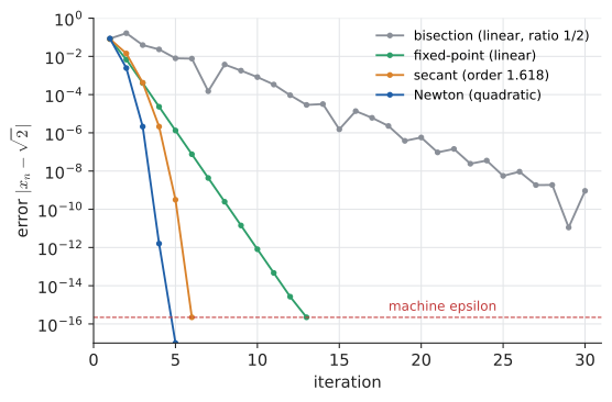
Each step halves the bracket, so after \(n\) steps the error is at most \((b-a)/2^{n}\). Reaching \(10^{-10}\) from a bracket of width 1 needs \(n\ge\log_2(10^{10})\approx33.2\), i.e. 34 steps. Linear convergence with ratio \(\tfrac12\): about one decimal digit every 3.3 steps.
32.5.4. Newton’s method: fast, demanding
Newton replaces the curve by its tangent line at \(x_n\) and jumps to where the tangent crosses zero:
For \(f(x)=x^2-2\) this is \(x_{n+1}=x_n-\dfrac{x_n^2-2}{2x_n} = \dfrac{x_n}{2}+\dfrac{1}{x_n}\). From \(x_0=1\):
The errors are \(8.6\times10^{-2}\), \(2.5\times10^{-3}\), \(2.1\times10^{-6}\), \(1.6\times10^{-12}\): the exponent roughly doubles each time. That is quadratic convergence. Step 5 hits the correctly rounded value of \(\sqrt2\). (Step 6 can bounce to the neighbouring double and back; at the level of the last bit, rounding decides, not Newton. Stopping tests must allow for that.)
Why quadratic? Expand \(f\) about the root with Taylor’s theorem: the tangent line captures the first-order term exactly, so the leftover error comes from the second-order term, which is proportional to \(e_n^2\). Precisely, \(e_{n+1}\approx \left|\dfrac{f''(r)}{2f'(r)}\right| e_n^2\).
32.5.5. The secant method: Newton without the derivative
Often \(f'\) is unavailable (\(f\) is a simulation, or a black box). Replace the tangent by the secant through the last two points, i.e. approximate \(f'(x_n)\) by \(\dfrac{f(x_n)-f(x_{n-1})}{x_n-x_{n-1}}\): Try it: Step the secant method.
From \(x_0=1, x_1=2\) (so \(f(x_0)=-1, f(x_1)=2\)):
Errors: \(8.1\times10^{-2}, 1.4\times10^{-2}, 4.2\times10^{-4}, 2.1\times10^{-6}, 3.2\times10^{-10}\). Each exponent is about 1.6 times the previous one: the order is the golden ratio \(p=\frac{1+\sqrt5}{2}\approx1.618\). Slower per step than Newton, but each step costs one new function evaluation instead of a function plus a derivative, so per unit of work the secant method is often faster.
32.5.6. Fixed-point iteration: the general pattern
Rewrite \(f(x)=0\) as \(x=g(x)\) and iterate \(x_{n+1}=g(x_n)\). A solution of \(x=g(x)\) is a fixed point of \(g\). Newton’s method is itself fixed-point iteration with \(g(x)=x-f(x)/f'(x)\). Try it: Watch x ← 2/x oscillate; Fixed point with cobweb.
Why it works. Near the fixed point \(r\), \(g(x_n)-g(r)\approx g'(r)(x_n-r)\), so \(e_{n+1}\approx|g'(r)|\,e_n\). The iteration converges (for starting points close enough) when \(|g'(r)|<1\), linearly with ratio \(|g'(r)|\), and the smaller \(|g'(r)|\), the faster.
Two rearrangements of \(x^2=2\):
-
\(g(x)=2/x\). Then \(g'(\sqrt2)=-2/2=-1\): the borderline. From \(x_0=1\) the iterates are \(2,1,2,1,\ldots\), oscillating forever.
-
\(g(x)=x-\tfrac13(x^2-2)\). Then \(g'(\sqrt2)=1-\tfrac23\sqrt2\approx0.0572\). From \(x_0=1\): \(1.\overline3,\ 1.4074,\ 1.41381,\ 1.414190,\ldots\), each error about 0.057 times the last, so about 1.24 digits per step; \(10^{-12}\) after 10 steps.
Fixed-point thinking reappears everywhere: Jacobi iteration below, PageRank (Chapter 28), value iteration in reinforcement learning, and the convergence proofs of many optimisers.
32.5.7. Choosing a method
| Method | Needs | Order \(p\) | Guaranteed? | Typical failure |
|---|---|---|---|---|
Bisection |
sign-change bracket |
1 (ratio \(\tfrac12\)) |
yes, if \(f\) continuous |
slow; cannot find double roots like \(x^2=0\) (no sign change) |
Fixed-point |
a rearrangement \(x=g(x)\) |
1 (ratio \(\lvert g'(r)\rvert\)) |
only if \(\lvert g'\rvert<1\) near root |
diverges or oscillates when \(\lvert g'(r)\rvert\ge1\) |
Secant |
two starting points |
1.618 |
no |
division by \(f(x_n)-f(x_{n-1})\approx0\); can wander off |
Newton |
\(f\) and \(f'\), one start |
2 |
no |
\(f'\approx0\); cycles; jumps to a far root; only linear at multiple roots |
Decision rule. If you can bracket the root and you only need it once, bisection’s certainty is worth its slowness. If you need the root to full precision, or millions of times, use a fast method, ideally safeguarded: production libraries (for example scipy.optimize.brentq) use Brent’s method, which tries secant-like and inverse-quadratic steps but falls back to bisection whenever a fast step would leave the bracket. You get guaranteed convergence and superlinear speed. Use Newton when derivatives are cheap and a good starting point is known (square roots in hardware, inside optimisers, implicit ODE solvers).
Here are all four, ready for experiments:
import math

def bisection(f, a, b, tol=1e-12):
    fa = f(a)
    while (b - a) / 2 > tol:
        m = (a + b) / 2
        fm = f(m)
        if fa * fm <= 0:
            b = m
        else:
            a, fa = m, fm
    return (a + b) / 2

def newton(f, df, x, tol=1e-12, max_iter=50):
    for _ in range(max_iter):
        step = f(x) / df(x)
        x -= step
        if abs(step) < tol:
            return x
    raise RuntimeError("Newton did not converge")

def secant(f, x0, x1, tol=1e-12, max_iter=50):
    for _ in range(max_iter):
        f0, f1 = f(x0), f(x1)
        if f1 == f0:
            break                     # flat secant: cannot continue
        x0, x1 = x1, x1 - f1 * (x1 - x0) / (f1 - f0)
        if abs(x1 - x0) < tol:
            break
    return x1

def fixed_point(g, x, tol=1e-12, max_iter=200):
    for _ in range(max_iter):
        x_new = g(x)
        if abs(x_new - x) < tol:
            return x_new
        x = x_new
    raise RuntimeError("fixed-point iteration did not converge")

f = lambda x: x*x - 2
print(bisection(f, 1, 2))
print(newton(f, lambda x: 2*x, 1.0))
print(secant(f, 1.0, 2.0))
print(fixed_point(lambda x: x - (x*x - 2)/3, 1.0))
print(math.sqrt(2))
1.4142135623724243 1.414213562373095 1.4142135623730951 1.4142135623730485 1.4142135623730951
Bisection and fixed-point iteration stop once their steps fall below \(10^{-12}\), so they agree with \(\sqrt2\) to about 12 digits, exactly as their tolerances promise. Secant reaches the correctly rounded value; Newton finishes one ulp below it (the last-bit bounce mentioned earlier). Each method delivers what its stopping test asked for, and no more.
|
Stopping criteria
"Stop when \(|f(x_n)|<\tau\)" is fragile: if \(f\) is very flat near the root, \(|f|\) is tiny far from it; if it is very steep, \(|f|\) may never get below \(\tau\) because of rounding. "Stop when \(|x_{n+1}-x_n|<\tau\)" is better but should use a relative tolerance for large roots (an absolute tolerance of \(10^{-12}\) is below the ulp of \(10^{6}\)). Always cap the number of iterations. |
|
Newton’s basins
Plot \(f(x)=x^3-2x+2\) and drag the starting point for Newton’s method. From \(x_0=0\) the iterates cycle \(0\to1\to0\to\ldots\) forever. Colour each starting point by which root (if any) it reaches, then switch to the complex plane (Chapter 15) for \(z^3-1=0\) and watch the famous fractal Newton basins appear. |
32.5.8. Where you’d use this
-
Everyday finance: what is this loan really costing? Borrow £10,000 and repay £880 a month for 12 months: £10,560 in all, which a salesperson might call a "5.6% flat rate". The true monthly rate \(r\) solves \(880\,\frac{1 - (1 + r)^{-12}}{r} = 10\,000\), which has no algebraic solution. Bisection or Newton gives \(r \approx 0.848\%\) a month, an effective annual rate of \(1.00848^{12} - 1 \approx 10.7\%\), nearly double the flat rate. Spreadsheet functions
RATEandIRRare root finders. -
Physics: Kepler’s equation. To find where a planet or satellite is at time \(t\), you must solve \(M = E - e\sin E\) for the angle \(E\), given the mean anomaly \(M\) and the eccentricity \(e\). Every orbit-prediction program (including the one in your phone’s GPS chip, which needs satellite positions) does this with a few Newton steps.
-
Engineering: the Colebrook equation for friction in a pipe, the equilibrium of a chemical reaction, and the operating point of a diode circuit are all "solve \(f(x) = 0\)" problems handed to a root finder.
32.6. Numerical differentiation: the V-shaped error
32.6.1. The problem
You have a function as code, say a physics simulation or a pricing model, and need its derivative. The definition (Chapter 17) suggests taking a small \(h\):
Mathematics says "the smaller \(h\) the better". The computer disagrees.
32.6.2. Intuition: two errors pulling in opposite directions
Truncation error comes from using a finite \(h\) instead of a limit. Taylor’s theorem (the polynomial approximation of Chapter 18) says
so
Truncation error is proportional to \(h\): it shrinks as \(h\) shrinks.
Rounding error comes from the subtraction \(f(x+h)-f(x)\): two nearly equal numbers, each carrying a rounding error of about \(u|f(x)|\). That is catastrophic cancellation again. The absolute error of the numerator is about \(u|f(x)|\), and we then divide by \(h\), giving an error of about \(u|f(x)|/h\), which grows as \(h\) shrinks.
32.6.3. Why it works: finding the best \(h\)
Total error is approximately
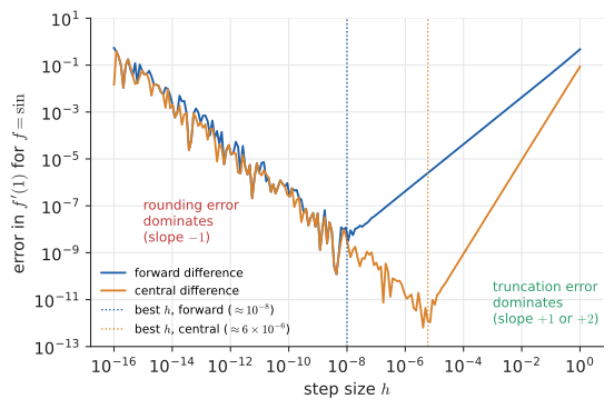
Minimise with calculus: \(E'(h)=\tfrac{M}{2}-\tfrac{u|f|}{h^2}=0\) gives \(h^\ast=\sqrt{2u|f|/M}\), which is of order \(\sqrt{u}\approx10^{-8}\) when \(f\) and \(f''\) are of order 1. At that \(h\) both terms are about \(10^{-8}\): the forward difference can only ever deliver about half the available digits.
The central difference is smarter. Subtract the Taylor expansions of \(f(x+h)\) and \(f(x-h)\); the \(f''\) terms cancel:
Truncation error is now \(O(h^2)\). Balancing \(h^2\) against \(u/h\) gives \(h^\ast\sim u^{1/3}\approx 6\times10^{-6}\) and a best error around \(u^{2/3}\approx10^{-11}\): about two-thirds of the digits.
|
Big-O notation for errors
\(E(h) = O(h^p)\) as \(h\to0\) means \(|E(h)|\le C h^p\) for some constant \(C\) and all small enough \(h\). A method with error \(O(h^p)\) has order \(p\): halving \(h\) divides the error by about \(2^p\). This is the same symbol as in algorithm analysis, but there \(n\to\infty\); here \(h\to0\). |
32.6.4. Worked example
Take \(f(x)=\sin x\) at \(x=1\), where the true derivative is \(\cos1 = 0.5403023058681398\). Try it: Plot the V-shaped error.
| \(h\) | forward | forward error | central | central error |
|---|---|---|---|---|
\(10^{-1}\) |
0.4973637525 |
\(4.3\times10^{-2}\) |
0.5394022522 |
\(9.0\times10^{-4}\) |
\(10^{-2}\) |
0.5360859810 |
\(4.2\times10^{-3}\) |
0.5402933009 |
\(9.0\times10^{-6}\) |
\(10^{-4}\) |
0.5402602314 |
\(4.2\times10^{-5}\) |
0.5403023050 |
\(9.0\times10^{-10}\) |
\(10^{-6}\) |
0.5403018851 |
\(4.2\times10^{-7}\) |
0.5403023059 |
\(2.8\times10^{-11}\) |
\(10^{-8}\) |
0.5403022918 |
\(1.4\times10^{-8}\) |
0.5403023029 |
\(3.0\times10^{-9}\) |
\(10^{-10}\) |
0.5403022474 |
\(5.8\times10^{-8}\) |
0.5403022474 |
\(5.8\times10^{-8}\) |
\(10^{-12}\) |
0.5403455461 |
\(4.3\times10^{-5}\) |
0.5402900349 |
\(1.2\times10^{-5}\) |
Read the forward column top to bottom: the error falls by a factor of 10 each time \(h\) does (order 1), bottoms out near \(h=10^{-8}\), then rises again. The central column falls by a factor of 100 per decade of \(h\) (order 2), bottoms out near \(h=10^{-6}\), then rises. Plot the error against \(h\) on log–log axes and you get the characteristic V.
32.6.5. Alternative approaches
-
Complex-step differentiation. If \(f\) is built from operations that make sense for complex numbers (Chapter 15), then \(f(x+ih)\approx f(x)+ihf'(x)\), so \(f'(x)\approx\operatorname{Im}f(x+ih)/h\). No subtraction occurs, so there is no cancellation and \(h\) can be absurdly small. With \(h=10^{-20}\),
cmath.sin(1 + 1e-20j).imag / 1e-20returns0.5403023058681398, correct to every digit. Try it: Try the complex step. -
Automatic differentiation (next sidebar) gives exact derivatives of code, to rounding error, with no \(h\) at all.
-
Symbolic differentiation (a computer algebra system) gives a formula, which is ideal when \(f\) is a formula, impossible when it is a 10,000-line simulation.
|
Halving \(h\)
A slider sets \(\log_{10}h\) from 0 to \(-16\). Show the secant line on the graph of \(f\), the computed slope, and a live point moving along the V-shaped error plot. Switch between forward, central and complex-step formulas and switch the precision between float16, float32 and float64 to see the bottom of the V move. Try it: Halving h in three precisions |
32.6.6. Where you’d use this
-
Sport and fitness trackers. A GPS watch records your position once a second and estimates your speed by a difference quotient. Position errors of a few metres divided by a 1-second step give speed errors of several metres per second, so the raw pace jumps about; watches smooth over several seconds, a larger \(h\), trading a little truncation error for much less noise. That is the V-shaped trade-off, with measurement noise in place of rounding.
-
Engineering: acceleration from measured velocity, flow rate from tank-level readings and the slope of a road from survey heights are all finite differences of noisy data; the larger the noise, the larger the best \(h\).
32.7. Numerical integration
32.7.1. The problem
Many integrals have no elementary antiderivative: \(\int e^{-x^2}dx\) (the normal distribution, Chapter 30), \(\int\sqrt{1+\cos^2x}\,dx\) (arc length of a sine wave), and every integral of measured data. The Riemann sums of Chapter 19 converge, but slowly. Can we do better with the same number of function evaluations?
As a test integral with a known answer we use
32.7.2. Intuition and derivation
Split \(\lbrack a,b\rbrack\) into \(n\) strips of width \(h=(b-a)/n\), with nodes \(x_i=a+ih\).
Trapezoid rule. Replace the curve on each strip by the straight line joining its endpoints. Each strip is a trapezoid with area \(\tfrac h2(f(x_{i})+f(x_{i+1}))\). Adding them, every interior node is counted twice:
The error is \(-\dfrac{(b-a)h^2}{12}f''(\xi)\) for some \(\xi\): order 2. (The sign tells you something too: for a convex function, \(f''>0\), the chords lie above the curve and the trapezoid rule overestimates.)
Simpson’s rule. Replace the curve on each pair of strips by the parabola through three points. Integrating that parabola (an exercise in Chapter 19-style algebra) gives weights \(\tfrac h3(1,4,1)\) on each pair, and adding pairs (\(n\) even):
The error is \(-\dfrac{(b-a)h^4}{180}f^{(4)}(\xi)\): order 4. Surprisingly, it is exact for cubics, not just quadratics, because the cubic error term is odd about each pair’s midpoint and cancels.
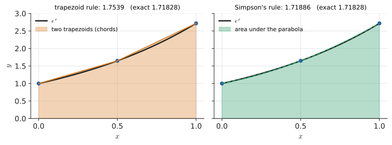
32.7.3. Worked example: \(n=2\) by hand
With \(n=2\), \(h=0.5\), nodes \(0,0.5,1\):
Trapezoid:
Error \(1.7539310925-1.7182818285=0.0356\), an overestimate, as predicted for convex \(e^x\).
Simpson:
Error \(5.8\times10^{-4}\), sixty times smaller with the same three function values.
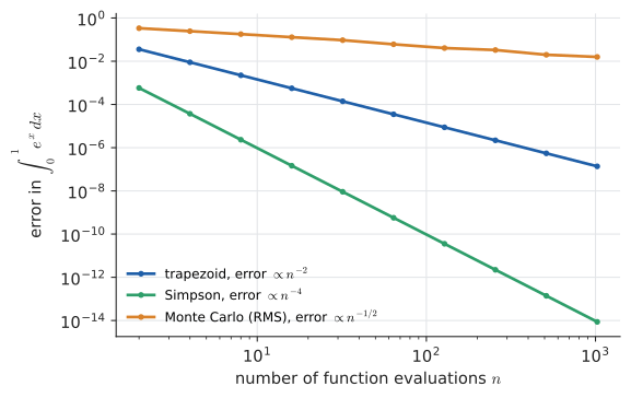
Doubling \(n\) repeatedly confirms the orders:
| \(n\) | \(T_n\) | error | \(S_n\) | error |
|---|---|---|---|---|
2 |
1.7539310925 |
\(3.6\times10^{-2}\) |
1.7188611519 |
\(5.8\times10^{-4}\) |
4 |
1.7272219046 |
\(8.9\times10^{-3}\) |
1.7183188419 |
\(3.7\times10^{-5}\) |
8 |
1.7205185922 |
\(2.2\times10^{-3}\) |
1.7182841547 |
\(2.3\times10^{-6}\) |
16 |
1.7188411286 |
\(5.6\times10^{-4}\) |
1.7182819741 |
\(1.5\times10^{-7}\) |
Trapezoid errors drop by a factor of 4 (\(=2^2\)) per doubling; Simpson errors by 16 (\(=2^4\)).
32.7.4. Alternative: Monte Carlo integration
A completely different idea from probability (Chapter 29): the average value of \(f\) on \(\lbrack a,b\rbrack\) is \(\frac{1}{b-a}\int_a^b f\), so pick \(n\) uniformly random points and average:
By the central limit theorem (Chapter 30) the error is random with standard deviation \(\sigma/\sqrt n\), where \(\sigma\) is the standard deviation of \(f(U)\). To gain one decimal digit you need 100 times as many points. Dreadful in one dimension, as the plot shows. But the \(1/\sqrt n\) rate does not depend on the dimension, whereas a grid-based rule in \(d\) dimensions with \(m\) points per axis needs \(m^d\) evaluations. For a 10-dimensional integral (pricing a basket option, rendering a pixel with light bouncing several times), Monte Carlo wins easily.
import math, random

def trapezoid(f, a, b, n):
    h = (b - a) / n
    return h * (f(a)/2 + sum(f(a + i*h) for i in range(1, n)) + f(b)/2)

def simpson(f, a, b, n):
    if n % 2:
        raise ValueError("Simpson's rule needs an even number of strips")
    h = (b - a) / n
    odd  = sum(f(a + i*h) for i in range(1, n, 2))
    even = sum(f(a + i*h) for i in range(2, n, 2))
    return h / 3 * (f(a) + 4*odd + 2*even + f(b))

def monte_carlo(f, a, b, n, rng=random.Random(42)):
    return (b - a) * sum(f(rng.uniform(a, b)) for _ in range(n)) / n

exact = math.e - 1
for n in (4, 16, 64):
    print(n, trapezoid(math.exp, 0, 1, n) - exact,
             simpson(math.exp, 0, 1, n) - exact,
             monte_carlo(math.exp, 0, 1, n) - exact)
4 0.008940076098471472 3.7013462701906974e-05 -0.34643844509874033 16 0.000559300120949402 1.4559284666759709e-07 -0.14119251170139946 64 3.495839104905585e-05 5.689697601951593e-10 0.0009426857183749693
32.7.5. Choosing a method
-
Smooth function, low dimension, can evaluate anywhere: Simpson, or better, an adaptive or Gaussian quadrature routine (
scipy.integrate.quad), which places points cleverly and estimates its own error. -
Data at fixed, equally spaced points (sensor readings): trapezoid or Simpson on the data you have.
-
Function with a kink or discontinuity: split the interval at the kink; higher-order rules lose their advantage across it.
-
Many dimensions, or a complicated region: Monte Carlo (or quasi-Monte Carlo with low-discrepancy sequences, which approaches \(1/n\)).
|
Higher order is not always better
Simpson’s error bound involves \(f^{(4)}\). If \(f\) is not smooth (\(\sqrt x\) near 0, \(|x|\), a step), the fourth derivative is huge or undefined and Simpson’s advantage evaporates; on \(\int_0^1\sqrt x\,dx\) both rules converge at only about order 1.5. Also, an error estimate is not an error guarantee: a function with a narrow spike between your sample points can fool any rule that only samples it. |
32.7.6. Where you’d use this
-
Medicine: drug exposure. Blood concentration of a drug measured at 0, 1, 2, 4, 6 and 8 hours is 0, 8, 10, 7, 4, 2 mg/L. The total exposure, the area under the curve (AUC), is estimated by the trapezoid rule on the unequal intervals: \(4 + 9 + 17 + 11 + 6 = 47\) mg·h/L. Regulators compare generic and brand-name drugs by exactly this number.
-
Everyday: area of an irregular garden or field. Measure the width every 2 m along its length and apply the trapezoid or Simpson rule: the method surveyors and builders use for lawns, ponds and cut-and-fill earthworks.
-
Physics and engineering: the energy used by a device is the integral of the power readings from a smart meter; the distance travelled by a car is the integral of its speedometer log; the impulse of a collision is the integral of a sampled force.
32.8. Solving linear systems on a computer
32.8.1. The problem
Systems \(A\mathbf x=\mathbf b\) with thousands or millions of unknowns arise in structural engineering, circuit simulation, least-squares fitting (Chapter 33), and the discretisation of every partial differential equation. You know Gaussian elimination from Chapter 6 and Chapter 27. What changes when it runs in floating point?
32.8.2. Why pivoting is essential
Solve Try it: Eliminate with a 10⁻²⁰ pivot.
The exact solution is extremely close to \(x=1, y=1\). Naive elimination uses the tiny \(10^{-20}\) as the pivot: multiply row 1 by \(m=1/10^{-20}=10^{20}\) and subtract from row 2:
\(x=0\) is completely wrong. The huge multiplier swamped row 2’s information (the "1" and "2" were rounded away), and the back substitution then divided a cancellation error by a tiny number.
Partial pivoting swaps the rows first so that the pivot is the largest entry (in absolute value) in its column:
Now the multiplier is \(10^{-20}\), at most 1 in size, and nothing gets swamped. With partial pivoting every multiplier satisfies \(|m|\le1\), which keeps the growth of rounding errors under control; in practice Gaussian elimination with partial pivoting is backward stable.
|
Pivot
In Gaussian elimination the pivot is the entry used to eliminate the entries below it in the same column. Partial pivoting chooses, at each column, the row with the largest absolute value in that column (among the rows not yet used) and swaps it into the pivot position. Back substitution solves the resulting upper-triangular system from the last equation upward. |
Input: an \(n\times n\) matrix \(A\) and vector \(\mathbf b\) (as the augmented matrix \(\lbrack A\mid\mathbf b\rbrack\)).
Steps:
-
For each column \(k=1,\ldots,n-1\):
-
Find the row \(p\ge k\) with the largest \(|a_{pk}|\). If it is zero, the matrix is singular; stop.
-
Swap rows \(p\) and \(k\).
-
For each row \(i>k\): compute the multiplier \(m_{ik}=a_{ik}/a_{kk}\) and replace row \(i\) by row \(i\) minus \(m_{ik}\) times row \(k\).
-
-
Back substitution: for \(i=n,n-1,\ldots,1\), set \(x_i = \big(b_i-\sum_{j>i}a_{ij}x_j\big)/a_{ii}\).
Output: the solution \(\mathbf x\). Cost: about \(\tfrac23n^3\) floating-point operations.
32.8.3. Worked example
Solve
Column 1. The entries are \(2,-3,-2\); the largest in absolute value is \(-3\) (row 2). Swap rows 1 and 2:
Multipliers: \(m_{21}=2/(-3)=-\tfrac23\), \(m_{31}=-2/(-3)=\tfrac23\).
Column 2. Among rows 2 and 3 the entries are \(\tfrac13\) and \(\tfrac53\); pivot on \(\tfrac53\), so swap rows 2 and 3. Multiplier \(m_{32}=\tfrac13\big/\tfrac53=\tfrac15\):
The triangular system is
Back substitution.
Check in the original first equation: \(2(2)+3-(-1)=8\). Correct.
import numpy as np

def solve_pp(A, b):
    """Gaussian elimination with partial pivoting, then back substitution."""
    A = np.array(A, dtype=float)
    b = np.array(b, dtype=float)
    n = len(b)
    for k in range(n - 1):
        p = k + np.argmax(np.abs(A[k:, k]))       # row of largest pivot
        if A[p, k] == 0:
            raise ValueError("matrix is singular")
        A[[k, p]], b[[k, p]] = A[[p, k]], b[[p, k]]  # swap rows k and p
        for i in range(k + 1, n):
            m = A[i, k] / A[k, k]
            A[i, k:] -= m * A[k, k:]
            b[i] -= m * b[k]
    x = np.zeros(n)
    for i in range(n - 1, -1, -1):
        x[i] = (b[i] - A[i, i+1:] @ x[i+1:]) / A[i, i]
    return x

print(solve_pp([[2, 1, -1], [-3, -1, 2], [-2, 1, 2]], [8, -11, -3]))
print(solve_pp([[1e-20, 1], [1, 1]], [1, 2]))
[ 2. 3. -1.] [1. 1.]
In practice call numpy.linalg.solve, which calls the LAPACK library’s pivoted LU factorisation. Never compute \(A^{-1}\) and multiply by it: that costs about three times as much and is less accurate.
32.8.4. Iterative methods: Jacobi
For a sparse system with a million unknowns, each equation involving only a handful of neighbours (a grid in a heat-flow simulation, links in a web graph), elimination is hopeless: it fills in the zeros and costs \(\sim n^3\). Iterative methods instead start from a guess and improve it, touching only the nonzero entries each sweep.
Jacobi’s idea: solve equation \(i\) for unknown \(i\), using the previous values of all the others. For
Start from \((x_0,y_0)=(0,0)\):
The iterates spiral in on the exact solution \((2,1)\); by \(k=8\) they read \((1.99990, 0.99995)\). Each sweep shrinks the error by a roughly constant factor (here about \(1/\sqrt{12}\approx0.29\)): linear convergence, exactly the fixed-point iteration of the root-finding section in vector form.
When does it converge? A sufficient condition is that \(A\) is strictly diagonally dominant: in each row, the diagonal entry is larger in absolute value than the sum of the absolute values of the others (\(4>1\), \(3>1\) above). Swap the equations to \(x+3y=5,\ 4x+y=9\) and Jacobi diverges.
Input: \(A\) (ideally strictly diagonally dominant), \(\mathbf b\), an initial guess \(\mathbf x^{(0)}\), a tolerance.
Steps:
-
For each \(i\), compute \(x_i^{(k+1)} = \big(b_i - \sum_{j\ne i}a_{ij}x_j^{(k)}\big)/a_{ii}\), using only old values.
-
Stop when \(\|\mathbf x^{(k+1)}-\mathbf x^{(k)}\|\) (or the residual \(\|A\mathbf x^{(k+1)}-\mathbf b\|\)) is below tolerance, or after a maximum number of sweeps.
Output: an approximate solution \(\mathbf x\).
Gauss–Seidel uses each new value as soon as it is computed and typically converges about twice as fast; conjugate gradient (for symmetric positive-definite \(A\)) and GMRES are the modern workhorses.
import numpy as np

def jacobi(A, b, x0=None, tol=1e-10, max_iter=500):
    A, b = np.asarray(A, float), np.asarray(b, float)
    D = np.diag(A)                       # diagonal entries
    R = A - np.diagflat(D)               # off-diagonal part
    x = np.zeros_like(b) if x0 is None else np.asarray(x0, float)
    for k in range(1, max_iter + 1):
        x_new = (b - R @ x) / D
        if np.linalg.norm(x_new - x, np.inf) < tol:
            return x_new, k
        x = x_new
    raise RuntimeError("Jacobi did not converge")

print(jacobi([[4, 1], [1, 3]], [9, 5]))
(array([2., 1.]), 21)
32.8.5. Where you’d use this
-
Electronics: circuit simulators (SPICE and its descendants) write Kirchhoff’s laws for every node of a circuit as one linear system and solve it with pivoted elimination, thousands of times per simulated microsecond.
-
Structural engineering: the finite-element model of a bridge or aircraft wing has a linear system with millions of unknowns (the displacements of mesh points). Its matrix is sparse and symmetric, so engineers use iterative solvers in the Jacobi family rather than elimination.
-
Medicine: a CT scanner reconstructs a cross-section of the body from X-ray measurements; each pixel is an unknown and each ray an equation. The first scanners solved this system with an iterative method (the algebraic reconstruction technique) in the same spirit as Jacobi.
32.9. Solving differential equations: Euler, RK4 and energy drift
32.9.1. The problem
Mechanics students learn Newton’s second law: force equals mass times acceleration. For a pendulum of length \(L\) swinging through angle \(\theta(t)\) this gives
For small swings, \(\sin\theta\approx\theta\) and the solution is a cosine (Chapter 13). For large swings there is no elementary formula. Planetary orbits, epidemics, circuits and chemical reactions are the same story: an equation for the rate of change of a state, and no formula for the state itself. We step forward in time instead.
|
Differential equation, initial value problem
A differential equation relates an unknown function to its derivatives. An initial value problem (IVP) gives \(\mathbf y'(t) = F(t,\mathbf y)\) together with a starting value \(\mathbf y(t_0)=\mathbf y_0\). Any higher-order equation becomes a first-order system by adding variables: for the pendulum take the state \(\mathbf y=(\theta,\omega)\) with angular velocity \(\omega=\theta'\), so \(\theta'=\omega,\ \omega'=-\tfrac gL\sin\theta\). The step size \(h\) is the time increment between computed states. |
32.9.2. Euler’s method: follow the tangent
Intuition. \(F(t,y)\) tells you the slope of the solution right now. Walk in that direction for a time \(h\), then look again:
It is the tangent-line approximation of Chapter 17 applied over and over.
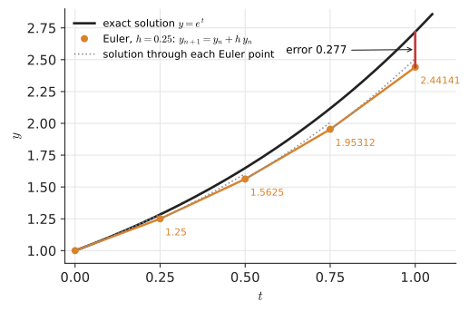
By hand. Take \(y'=y,\ y(0)=1\), whose exact solution is \(e^t\), and step to \(t=1\) with \(h=0.25\): Try it: Try Euler with h = 0.25.
The true value is \(e = 2.71828\); Euler is low by 0.277 because the slope keeps increasing during each step and Euler always uses the stale slope from the start. (Notice that \(y_4=1.25^4\): Euler computes \((1+h)^{1/h}\), the compound-interest approximation of \(e\) from Chapter 12.) With \(h=0.1, 0.01, 0.001\) the errors are \(0.125, 0.0135, 0.00136\): the error is proportional to \(h\). Euler is a first-order method; for six correct digits you would need about a million steps.
32.9.3. Runge–Kutta 4: sample the slope four times
Intuition. Instead of trusting the slope at the start of the step, probe it at the start, twice at the midpoint, and at the end, and take a weighted average, in exactly the proportions of Simpson’s rule (\(1:2:2:1\) is \(1:4:1\) with the middle weight split):
By hand, one step of \(y'=y\), \(y_0=1\), \(h=0.25\):
The exact value is \(e^{0.25}=1.2840254\). One RK4 step is already correct to 5 digits, where Euler’s first step (1.25) was correct to 1. Four steps reach \(t=1\) with error \(7.2\times10^{-5}\), compared to Euler’s 0.277. RK4 is fourth order: halve \(h\) and the error falls by 16. It costs four evaluations of \(F\) per step, but that is a bargain.
Input: \(F(t,\mathbf y)\), initial state \(\mathbf y_0\) at \(t_0\), step \(h\), number of steps \(N\).
Steps: for \(n=0,1,\ldots,N-1\), compute \(k_1,k_2,k_3,k_4\) as above (each a vector if the state is a vector), set \(\mathbf y_{n+1}=\mathbf y_n+\tfrac h6(k_1+2k_2+2k_3+k_4)\) and \(t_{n+1}=t_n+h\).
Output: the approximate trajectory \(\mathbf y_0,\mathbf y_1,\ldots,\mathbf y_N\).
32.9.4. Experiment: energy drift in a pendulum
A frictionless pendulum conserves energy: per unit mass and with \(g/L=1\), Try it: Run the energy-drift experiment.
(kinetic plus potential) is constant forever. Energy therefore makes a superb diagnostic: any drift in \(E\) is pure numerical error. Release the pendulum from rest at \(\theta=1\) radian and simulate 60 time units with \(h=0.1\), using Euler, RK4, and a third contender, the semi-implicit (symplectic) Euler method, which differs from Euler only in updating the velocity first and then using the new velocity to update the position:
import math

def accel(theta):
    return -math.sin(theta)          # g/L = 1

def energy(theta, omega):
    return 0.5 * omega**2 + (1 - math.cos(theta))

def euler_step(th, om, h):
    return th + h * om, om + h * accel(th)

def semi_implicit_step(th, om, h):
    om = om + h * accel(th)          # update velocity first...
    return th + h * om, om           # ...then use the NEW velocity

def rk4_step(th, om, h):
    k1t, k1o = om,              accel(th)
    k2t, k2o = om + h/2 * k1o,  accel(th + h/2 * k1t)
    k3t, k3o = om + h/2 * k2o,  accel(th + h/2 * k2t)
    k4t, k4o = om + h * k3o,    accel(th + h * k3t)
    return (th + h/6 * (k1t + 2*k2t + 2*k3t + k4t),
            om + h/6 * (k1o + 2*k2o + 2*k3o + k4o))

def simulate(step, h=0.1, t_end=60.0):
    th, om = 1.0, 0.0                # released from rest at 1 radian
    E0 = energy(th, om)
    for _ in range(round(t_end / h)):
        th, om = step(th, om, h)
    return energy(th, om) / E0

for name, step in [("Euler", euler_step),
                   ("semi-implicit", semi_implicit_step),
                   ("RK4", rk4_step)]:
    print(f"{name:14s} E(60)/E(0) = {simulate(step):.6f}")
Try it: Run this in your browser.
Euler          E(60)/E(0) = 8.123523
semi-implicit  E(60)/E(0) = 1.021577
RK4            E(60)/E(0) = 0.999994
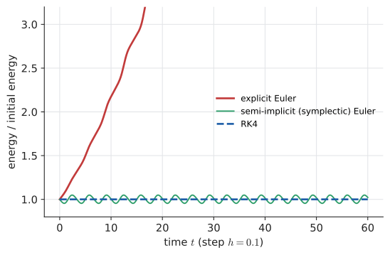
Three very different personalities:
-
Explicit Euler pumps energy in at every step: after 60 time units the pendulum has eight times its starting energy and is whirling over the top. Smaller \(h\) slows the drift (with \(h=0.01\) the ratio is 1.62 at \(t=60\)) but never stops it.
-
RK4 is far more accurate per step and the energy looks perfectly flat on this plot. Over very long runs it slowly leaks energy (ratio 0.9994 after 6000 time units): small, but systematic.
-
Semi-implicit Euler is only first order, so its energy wobbles visibly, by up to about 5% at this step size, but the wobble stays bounded forever (still within 5% of the starting energy throughout 6000 time units). It belongs to the family of symplectic integrators, which exactly preserve a nearby "shadow" energy and therefore cannot drift.
The lesson: order of accuracy is not the only virtue. For long simulations of conservative systems (planetary orbits over millions of years, molecular dynamics, game physics), preserving the right structure beats raw accuracy per step.
|
Stiffness
Some systems mix very fast and very slow processes (a chemical reaction with a microsecond and an hour time scale). Explicit methods like Euler and RK4 must then use a step size dictated by the fastest process, even after it has died away, or they blow up. Such systems are stiff and need implicit methods (backward Euler, BDF), which solve an equation (often with Newton’s method) at each step. If your ODE solver crawls or explodes, suspect stiffness and try |
|
Orbits and drift
Before symplectic methods, long-term solar-system simulations showed planets slowly spiralling into the Sun or escaping, purely from integrator error. Symplectic integrators such as Wisdom–Holman (1991) made billion-year simulations credible, and with them the discovery that the inner solar system is chaotic: Mercury’s orbit cannot be predicted beyond a few tens of millions of years. |
|
Integrator shoot-out
Animate three pendulums side by side, one per integrator, with a live energy trace underneath. Sliders control \(h\) and the release angle. Then switch to a planet orbiting a star and watch Euler’s orbit spiral outward while the symplectic orbit precesses but stays closed. Try it: Open the integrator shoot-out |
32.9.5. Where you’d use this
-
Everyday: a cooling cup of tea. Newton’s law of cooling, \(T' = -0.1(T - 20)\) (per minute, room at 20 °C), with tea at 90 °C. Two Euler steps of one minute: \(T_1 = 90 - 0.1 \times 70 = 83\), \(T_2 = 83 - 0.1 \times 63 = 76.7\). The exact answer \(20 + 70e^{-0.2} \approx 77.3\) °C shows Euler’s typical first-order lag; RK4 with the same step agrees to four decimal places.
-
Medicine and public health: epidemic models (the SIR equations for susceptible, infected and recovered people) are integrated step by step to forecast hospital demand; pharmacologists integrate drug-absorption models to set dosing intervals.
-
Engineering and science: weather and climate models, spacecraft trajectories, the charging of a capacitor in a circuit simulator, and every "physics" step in a game are numerical ODE solutions; the choice of integrator decides whether they stay stable over long runs.
32.10. Adding up a long list: Kahan summation
32.10.1. The problem
Add 0.1 to itself ten million times. The answer should be 1,000,000. Try it: Add 0.1 ten million times.
s = 0.0
for _ in range(10_000_000):
    s += 0.1
print(s)
999999.9998389754
Not only is 0.1 inexact, but once the running sum is large each addition rounds the tiny increment to the ulp of the sum, and the rounding errors accumulate. For naive summation of \(n\) terms the error bound grows like \(n\,u\sum|x_i|\): with \(n=10^7\) that is a loss of 7 of the 16 digits in the worst case.
32.10.2. Intuition: keep the change
Imagine a cash register that can only display four significant digits. The total is 1000; a customer adds a 0.4 item; the register shows 1000 again and the 0.4 vanishes. Ten such items vanish entirely: the register says 1000 when the truth is 1004. A sensible cashier would keep the lost amounts in a jar and add them back in when they became big enough to register. That jar is Kahan’s compensation variable. Try it: Run the cash register.
Here is the cash register in Python, using the decimal module set to 4 significant digits so we can watch every step:
from decimal import Decimal as D, getcontext
getcontext().prec = 4                       # a 4-digit "computer"

xs = [D(1000)] + [D("0.4")] * 10            # true sum: 1004

s = D(0)
for x in xs:
    s = s + x
print("naive:", s)

s, c = D(0), D(0)
for x in xs:
    y = x - c                                # add back what was lost last time
    t = s + y
    c = (t - s) - y                          # what was lost this time (negated)
    s = t
print("Kahan:", s)
naive: 1000 Kahan: 1004
Trace the first few Kahan steps after the sum reaches 1000:
| term | \(y = x - c\) | \(t = \mathrm{fl}(s+y)\) | \(c = (t-s)-y\) | new \(s\) |
|---|---|---|---|---|
0.4 |
\(0.4-0=0.4\) |
\(\mathrm{fl}(1000.4)=1000\) |
\((1000-1000)-0.4=-0.4\) |
1000 |
0.4 |
\(0.4-(-0.4)=0.8\) |
\(\mathrm{fl}(1000.8)=1001\) |
\((1001-1000)-0.8=0.2\) |
1001 |
0.4 |
\(0.4-0.2=0.2\) |
\(\mathrm{fl}(1001.2)=1001\) |
\((1001-1001)-0.2=-0.2\) |
1001 |
0.4 |
\(0.4-(-0.2)=0.6\) |
\(\mathrm{fl}(1001.6)=1002\) |
\((1002-1001)-0.6=0.4\) |
1002 |
\(c\) always holds the negative of the rounding error just committed (in \(t-s\), the part of \(y\) that actually made it into the sum, minus \(y\)). Algebraically \((t-s)-y=0\); in floating point it is exactly the lost low-order part. This is one of the rare places where you want the subtraction of nearly equal numbers, because here they are exact.
Input: a sequence of floating-point numbers \(x_1,\ldots,x_n\).
Steps:
-
Set the sum \(s\leftarrow0\) and the compensation \(c\leftarrow0\).
-
For each \(x_i\):
-
\(y\leftarrow x_i - c\) (correct the incoming term by the error from last time).
-
\(t\leftarrow s + y\) (low-order digits of \(y\) may be lost here).
-
\(c\leftarrow (t - s) - y\) (recover them, with a minus sign).
-
\(s\leftarrow t\).
-
Output: \(s\), with error bounded by about \(2u\sum|x_i|\) independent of \(n\) (plus a negligible \(O(nu^2)\) term).
import math

def naive_sum(xs):
    s = 0.0
    for x in xs:
        s += x
    return s

def kahan_sum(xs):
    s = 0.0          # running sum
    c = 0.0          # compensation: the low-order bits we lost last time
    for x in xs:
        y = x - c            # correct the next term by what we lost before
        t = s + y            # add; low-order digits of y may be lost here
        c = (t - s) - y      # recover what was lost (algebraically zero!)
        s = t
    return s

xs = [0.1] * 10_000_000
print(naive_sum(xs))
print(kahan_sum(xs))
print(math.fsum(xs))
999999.9998389754 1000000.0 1000000.0
32.10.3. Alternatives and choosing
-
math.fsumgoes further and returns the correctly rounded sum of the stored values (it tracks partial sums exactly). Use it in Python whenever accuracy matters. -
Pairwise summation adds in a balanced tree: error grows like \(\log_2 n\) instead of \(n\). NumPy’s
np.sumdoes this automatically for contiguous arrays, which is why it is usually more accurate than a Python loop. -
Sorting the terms by increasing magnitude before adding helps when they all have the same sign.
-
For a handful of numbers of similar size, naive summation is fine. Reach for compensated summation for long sums (statistics over large datasets, long simulations accumulating time, numerical integration with many points), and for sums with mixed magnitudes.
|
Compilers can "optimise" Kahan away
To an optimiser that assumes real-number algebra, \(c=(t-s)-y\) with \(t=s+y\) simplifies to \(c=0\). C and C++ compilers with |
|
Order of addition matters
Floating-point addition is commutative (\(a+b=b+a\)) but not associative: \((10^{20} + -10^{20}) + 1 = 1\), while \(10^{20} + (-10^{20} + 1) = 0\). This is why a parallel reduction on a GPU can give slightly different answers from run to run (threads finish in different orders), and why "bitwise reproducible" scientific codes go to great lengths to fix the order of summation. |
32.11. Interpolation: filling in between the points
32.11.1. The problem
You have values of a function only at a few points: a table of tax brackets, a few calibration measurements, keyframes of an animation. You need values in between. Interpolation finds a function that passes exactly through the given points and uses it to estimate the rest.
32.11.2. Lagrange’s formula: one polynomial through all the points
Through any two points there is exactly one line; through three points (with distinct \(x\)) exactly one parabola; through \(n+1\) points exactly one polynomial of degree at most \(n\) (Chapter 7). Lagrange’s idea writes it down directly. For nodes \(x_0,\ldots,x_n\), build basis polynomials that are 1 at their own node and 0 at all the others:
The \(\prod\) symbol is the product analogue of \(\sum\): multiply the factors for every \(j\) from 0 to \(n\) except \(j=i\). At \(x=x_i\) every factor equals 1; at any other node \(x_k\) the factor with \(j=k\) is zero. Then
passes through every data point, because at \(x_k\) only the \(k\)-th term survives and it equals \(y_k\).
Worked example. Find the polynomial through \((0,1),(1,3),(2,7)\) and estimate \(p(1.5)\).
Check: \(p(0)=1\), \(p(1)=3\), \(p(2)=7\). And \(p(1.5)=2.25+1.5+1=4.75\). (Directly from the basis values: \(L_0(1.5)=-0.125\), \(L_1(1.5)=0.75\), \(L_2(1.5)=0.375\), so \(p(1.5)=-0.125+2.25+2.625=4.75\).)
def lagrange(xs, ys, x):
    total = 0.0
    for i, (xi, yi) in enumerate(zip(xs, ys)):
        L = 1.0
        for j, xj in enumerate(xs):
            if j != i:
                L *= (x - xj) / (xi - xj)
        total += yi * L
    return total

print(lagrange([0, 1, 2], [1, 3, 7], 1.5))
4.75
32.11.3. Failure mode: Runge’s phenomenon
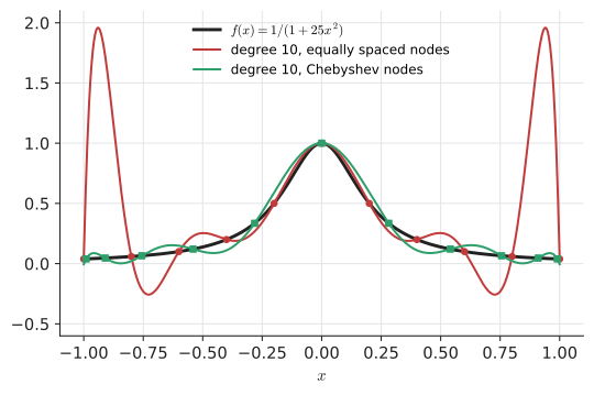
More points should mean a better fit. Carl Runge showed in 1901 that this is false. Interpolate \(f(x)=1/(1+25x^2)\) on \(\lbrack -1,1\rbrack\) at equally spaced points: Try it: See Runge’s wiggle; Same degree, Chebyshev nodes.
| degree | max error, equally spaced nodes | max error, Chebyshev nodes |
|---|---|---|
5 |
0.43 |
0.56 |
10 |
1.92 |
0.11 |
15 |
2.11 |
0.083 |
20 |
59.8 |
0.015 |
With equally spaced nodes the interpolant fits beautifully in the middle and oscillates wildly near the ends, and the oscillation grows with the degree. The cure is either to cluster the nodes near the ends, using Chebyshev nodes \(x_k=\cos\!\big(\tfrac{(2k+1)\pi}{2(n+1)}\big)\) (the projections onto the \(x\)-axis of equally spaced points on a semicircle), or to abandon a single high-degree polynomial altogether.
32.11.4. Choosing a method
-
Piecewise linear interpolation (join the dots): robust, never overshoots, but has corners. What
numpy.interpdoes. -
Cubic splines: a separate cubic on each interval, joined so that the first and second derivatives match. Smooth, local, no Runge oscillation. The default for smooth curves through data.
-
Single global polynomial: only for a few points, or with Chebyshev nodes when you get to choose where to sample.
-
If the data are noisy, do not interpolate at all: fit (least squares, Chapter 31, Chapter 33), because forcing a curve through every noisy point fits the noise.
|
Runge’s wiggle
Drag the number of nodes from 2 to 25 for \(1/(1+25x^2)\) and toggle between equally spaced and Chebyshev nodes, and between a global polynomial and a cubic spline. Then drag individual data points and see how far the disturbance spreads: everywhere for the global polynomial, only locally for the spline. Try it: Open Runge’s wiggle · Compare a cubic spline |
32.11.5. Where you’d use this
-
Everyday: a weather app knows forecast temperatures on a grid of points every few kilometres and every hour; the temperature "at your street at 2:30" is interpolated. If it’s 14 °C at 2 pm and 18 °C at 3 pm, linear interpolation gives 16 °C at 2:30.
-
Science and engineering: steam tables, tide tables and calibration tables for thermocouples are read by interpolation between tabulated values; a thermostat that converts sensor voltage to temperature through a lookup table interpolates every reading.
-
Computing: animation tweening, texture sampling in graphics (bilinear interpolation between texels), and audio resampling (changing 44.1 kHz to 48 kHz) are interpolation running millions of times a second.
32.12. When to trust a number
Every section of this chapter has shown a way in which a confident-looking 16-digit number can be wrong. Pulling the lessons together gives a practical discipline.
32.12.1. Sources of error, in one place
| Source | Example | What controls it |
|---|---|---|
Modelling error |
\(\sin\theta\approx\theta\); frictionless pendulum |
the science, not the numerics |
Data error |
measured inputs good to 3 digits |
conditioning: expect about \(\kappa\times\) data error |
Truncation (discretisation) error |
finite \(h\), finitely many terms or iterations |
the method’s order; refine \(h\) |
Rounding error |
53-bit arithmetic |
stability of the algorithm; avoid cancellation |
Bugs |
wrong sign, off-by-one in a loop |
tests against known answers |
The order matters. There is no point computing to 15 digits a model that is right to 2, or polishing rounding error when the step size is the dominant error.
Input: a computed result.
Steps:
-
Sanity: Are the units, sign and order of magnitude right? Do conserved quantities stay conserved? Does a probability lie in \(\lbrack 0,1\rbrack\)?
-
Known cases: Does the same code reproduce an answer you know exactly (a test problem like \(x^2-2\), \(\int_0^1 e^x\,dx\), a linear pendulum)?
-
Convergence: Halve the step size (or double the points, or tighten the tolerance). Does the answer change in the digits you care about? Does the change shrink at the rate the method’s order predicts?
-
Residual: For an equation, plug the answer back in. For \(A\mathbf x=\mathbf b\), is \(\|A\mathbf x-\mathbf b\|\) small? (A small residual with a large condition number still permits a large error.)
-
Conditioning: Perturb the inputs by their uncertainty. How much does the output move?
-
Independent method: Solve it another way (a different algorithm, a different library, higher precision with
decimalormpmath). Agreement between genuinely different methods is strong evidence.
Output: a result together with an honest estimate of how many of its digits mean something.
|
Precision is not accuracy
A double always prints with up to 17 significant digits. That says nothing about how many are correct. The forward recurrence for \(I_{20}\) printed |
32.13. Interactive tools
Browser tools on the companion website that go with this chapter. Each example link in the chapter opens one of them with that example already set up.
32.14. Exercises
-
Recognition. For each, name the kind of error that dominates (rounding, cancellation, truncation, overflow, underflow, instability, ill-conditioning): (a)
1e308 * 10; (b) multiplying 500 probabilities of 0.1; (c) forward difference with \(h=10^{-14}\); (d) Euler’s method with \(h=0.5\); (e) solving two nearly parallel lines from data measured to 3 digits. -
Convert 0.75 and 0.3 to binary. Which is stored exactly as a double, and why?
-
What is \(\mathrm{ulp}(2^{30})\) for a double? Can a double represent \(2^{30}+0.25\) exactly?
-
Evaluate \(\sqrt{x^2+1}-x\) for \(x=10^8\) naively in Python, then derive and test a cancellation-free rewrite.
-
Compute the condition number \(\kappa(x)=|xf'(x)/f(x)|\) of \(f(x)=\ln x\). Where is taking a logarithm ill-conditioned?
-
Perform three bisection steps and three Newton steps (from \(x_0=1\)) on \(f(x)=x^3-2\). How many correct digits does each have?
-
The fixed-point iteration \(x_{n+1}=\cos x_n\) solves \(x=\cos x\). Using \(g'(x)=-\sin x\) and the root \(r\approx0.739\), predict the convergence ratio, then check by experiment.
-
For \(f(x)=e^x\) at \(x=0\), the forward difference with \(h=0.1\) gives what value and what error? What does the error theory predict (\(\approx \tfrac h2 f''(x)\))?
-
Apply the trapezoid rule and Simpson’s rule with \(n=2\) to \(\int_0^2 x^3\,dx\). Explain why Simpson’s answer is exact.
-
Solve by Gaussian elimination with partial pivoting, showing each swap and multiplier: \(x+2y=5,\ 3x+4y=11\).
-
Problem solving. Use one step of Euler and one step of RK4 with \(h=0.1\) on \(y'=-2y,\ y(0)=1\). Compare with \(e^{-0.2}\). Then explain what happens to Euler if \(h=1.5\) and why (look at the multiplier per step).
-
Problem solving. Write a function that sums a list both naively and with Kahan’s algorithm, and find a list of ten numbers for which the naive float sum is off by at least 1. (Hint: mix \(10^{16}\) and 1.)
Answers
-
(a) overflow, result
inf; (b) underflow: \(10^{-500}\) is below \(4.9\times10^{-324}\), result 0.0 (use logs); (c) cancellation (rounding error amplified by \(1/h\)); (d) truncation; (e) ill-conditioning. -
\(0.75 = 0.11_2\) (exact, since \(0.75=3/4\) has a power-of-two denominator). \(0.3\): \(0.3\to0.6(0)\to1.2(1)\to0.4(0)\to0.8(0)\to1.6(1)\to1.2(1)\ldots\), so \(0.3=0.0\overline{1001}_2\), which never terminates (denominator 10 contains 5); it is rounded.
-
\(2^{30}=1.0\times2^{30}\), so \(\mathrm{ulp}=2^{30}\times2^{-52}=2^{-22}\approx2.4\times10^{-7}\). Since \(0.25=2^{-2}\) is a multiple of \(2^{-22}\), \(2^{30}+0.25\) is exact.
-
Naively,
math.sqrt(1e16+1) - 1e8gives0.0(\(10^{16}+1\) rounds to \(10^{16}\)). Multiply by the conjugate: \(\sqrt{x^2+1}-x=\dfrac{(x^2+1)-x^2}{\sqrt{x^2+1}+x}=\dfrac{1}{\sqrt{x^2+1}+x}\), which gives5e-09, correct to full precision (true value \(4.99999999999999999\ldots\times10^{-9}\)). -
\(f'(x)=1/x\), so \(\kappa=|x\cdot\frac1x/\ln x|=1/|\ln x|\). It blows up as \(x\to1\) (where \(\ln x\to0\)): computing \(\ln x\) for \(x\) near 1 is ill-conditioned, which is why
log1pexists. -
Bisection on \(\lbrack 1,2\rbrack\): \(m=1.5\) (\(f=1.375>0\), \(b=1.5\)); \(m=1.25\) (\(f=-0.047<0\), \(a=1.25\)); \(m=1.375\) (\(f=0.600>0\)). Bracket \(\lbrack 1.25,1.375\rbrack\), estimate 1.3125, about 1 correct digit (\(\sqrt[3]{2}=1.259921\)). Newton: \(x_{n+1}=x_n-(x_n^3-2)/(3x_n^2)\): \(x_1=1+1/3=1.3333\), \(x_2=1.3333-(2.3704-2)/5.3333=1.2639\), \(x_3=1.2599335\), correct to 4–5 digits (error \(1.2\times10^{-5}\)).
-
\(|g'(r)|=\sin(0.739)\approx0.674\). Each step multiplies the error by about 0.67, so about 0.17 digits per step; about 55 iterations from \(x_0=1\) to reach \(10^{-10}\). Experiment confirms successive error ratios near \(-0.674\) (the sign alternates, so the iterates zig-zag around the root).
-
\((e^{0.1}-1)/0.1 = 1.0517092\), error \(0.0517\). Prediction \(\tfrac{0.1}{2}e^0=0.05\); the remaining 0.0017 is the next Taylor term \(\tfrac{h^2}{6}\).
-
\(h=1\), values \(0,1,8\). Trapezoid: \(1\cdot(0+1+4)=5\). Simpson: \(\tfrac13(0+4+8)=4\). Exact: \(\int_0^2x^3dx=4\). Simpson is exact for cubics because its error term involves \(f^{(4)}\), which is zero.
-
Column 1: largest is 3, swap: \(3x+4y=11,\ x+2y=5\). Multiplier \(m=1/3\): row 2 becomes \((2-\tfrac43)y=5-\tfrac{11}3\), i.e. \(\tfrac23y=\tfrac43\), so \(y=2\). Back substitute: \(3x+8=11\), \(x=1\).
-
Euler: \(y_1=1+0.1(-2)=0.8\). RK4: \(k_1=-2\), \(k_2=-2(1-0.1)=-1.8\), \(k_3=-2(1-0.09)=-1.82\), \(k_4=-2(1-0.182)=-1.636\); \(y_1=1+\tfrac{0.1}6(-2-3.6-3.64-1.636)=1-\tfrac{1.0876}{6}=0.818733\). Exact \(e^{-0.2}=0.818731\). Euler error 0.019, RK4 error \(2.6\times10^{-6}\). With \(h=1.5\) Euler multiplies by \(1+h(-2)=-2\) each step: \(1,-2,4,-8,\ldots\), an oscillating explosion although the true solution decays. Euler is stable for this equation only when \(|1-2h|<1\), i.e. \(h<1\). This is stiffness in miniature.
-
Example:
[1e16, 1.0, 1.0, 1.0, 1.0, 1.0, 1.0, 1.0, 1.0, -1e16]. True sum 8. Naive: each1e16 + 1.0rounds back to1e16(ulp at \(10^{16}\) is 2, and ties round to even), so the result is0.0. Kahan returns8.0.
32.15. Mastery check
-
Explain in two sentences why
0.1 + 0.2 != 0.3in IEEE 754 doubles. -
State machine epsilon for doubles and what the model \(\mathrm{fl}(x\circ y)=(x\circ y)(1+\delta)\) says.
-
The expression \((1-\cos x)/x^2\) should approach \(\tfrac12\) as \(x\to0\). What does it return for \(x=10^{-8}\) in double precision, why, and how do you fix it?
-
Distinguish an ill-conditioned problem from an unstable algorithm, with one example of each.
-
Rank bisection, secant, Newton and fixed-point iteration by order of convergence, and give one situation where you would choose bisection anyway.
-
Why does the error of a forward-difference derivative first decrease and then increase as \(h\to0\)? Roughly what \(h\) is optimal in double precision?
-
Simpson’s rule with \(n\) strips has error 0.0008. Estimate the error with \(2n\) strips.
-
In a long orbital simulation, which would you prefer, RK4 or a symplectic method, and why?
Decision rule: All correct without hesitation → move on to Chapter 33. Stuck on 1–3 → reread Section 32.2 and Section 32.3. Stuck on 4–5 → reread Section 32.4 and Section 32.5. Stuck on 6–8 → reread Section 32.6, Section 32.7 and Section 32.9, then work the exercises in Section 32.14.
Mastery check answers
-
0.1, 0.2 and 0.3 have infinite binary expansions, so each is stored as the nearest double, with a tiny error. The rounding errors of 0.1 and 0.2 are both upward and their sum rounds to the double just above the stored 0.3.
-
\(\varepsilon_{\text{mach}}=2^{-52}\approx2.22\times10^{-16}\). Each basic operation returns the exact result rounded to nearest, so it is wrong by a relative amount at most \(u=2^{-53}\).
-
\(\cos(10^{-8})\) rounds to exactly 1, so the numerator is 0 and the result is 0.0 instead of 0.5: catastrophic cancellation. Rewrite as \(2\sin^2(x/2)/x^2\), which gives 0.5.
-
Ill-conditioned: the answer is sensitive to the data whatever algorithm you use (nearly parallel lines; \(\kappa\approx4\times10^4\)). Unstable: the algorithm amplifies rounding errors on a problem that is fine (the forward recurrence \(I_n=1-nI_{n-1}\); naive elimination without pivoting on the \(10^{-20}\) system).
-
Newton (2) > secant (about 1.618) > bisection and fixed-point (both 1; bisection’s ratio is \(\tfrac12\), fixed-point’s is \(|g'(r)|\)). Choose bisection when you have a sign-change bracket and need guaranteed convergence with no derivative, e.g. a one-off root of a black-box function, or as the safeguard inside Brent’s method.
-
Truncation error (proportional to \(h\)) falls as \(h\) shrinks, but cancellation in \(f(x+h)-f(x)\) produces a rounding error of about \(u|f|/h\) that grows. The optimum is near \(\sqrt u\approx10^{-8}\) (about \(10^{-5}\) to \(10^{-6}\) for central differences).
-
Simpson is fourth order: doubling \(n\) halves \(h\) and divides the error by \(2^4=16\), giving about \(5\times10^{-5}\).
-
A symplectic method (semi-implicit Euler, Verlet, Wisdom–Holman). RK4 is more accurate per step but its energy drifts systematically over long times, so orbits slowly decay or spread; symplectic methods keep energy errors bounded forever.