Volume 1: Foundations to Precalculus · Part II: Algebra
Chapter 8. Quadratics
Chapter map: the quadratic is the first equation in this book that cannot be solved by "undo each operation in turn", and the first function whose graph bends. It is also the best-studied object in elementary algebra, which makes it the ideal place to practise the habits this book cares about: seeing one object as words, symbols, a picture and a computation; knowing several methods and choosing between them; deriving the famous formula rather than memorising it; and knowing exactly when the formula, run on a real computer, gives the wrong answer. Quadratics are also the first non-linear model you meet in practice: anything accelerating, the area of a shape with one adjustable length, any "price times quantity", and any sum of squared errors is one.
8.1. Three problems that are secretly the same
8.1.1. A ball thrown upwards
You stand on a platform and throw a ball straight up. It leaves your hand 2 m above the ground, moving upwards at 15 m/s. When does it hit the ground? How high does it go?
If you did sixth-form mechanics, you met the constant-acceleration ("SUVAT") equations. The one that matters here is
where \(s\) is displacement, \(u\) initial velocity, \(a\) acceleration and \(t\) time. Measuring upwards, \(u = 15\) m/s and \(a = -9.8\) m/s² (gravity pulls down). Adding the 2 m starting height, the height after \(t\) seconds is
"When does it hit the ground?" becomes: solve \(2 + 15t - 4.9t^2 = 0\). The unknown appears both squared and unsquared. You cannot "subtract 2, then divide by 15" as you would for a linear equation, because the \(t^2\) term refuses to go away. You need a new idea.
8.1.2. A fence against a wall
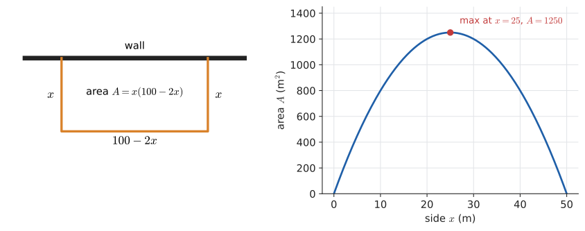
You have 100 m of fencing and want a rectangular pen against a long wall, so you only need to fence three sides. If the two sides perpendicular to the wall are \(x\) metres each, the side parallel to the wall is \(100 - 2x\), and the area is
Which \(x\) gives the biggest pen? Again a squared term, and this time the question is not "where is it zero?" but "where is it largest?"
8.1.3. Breaking even
A small company finds that, selling \(q\) hundred units a month, its profit in thousands of pounds is
At low volume, fixed costs swamp revenue; at very high volume, it has to cut prices so far that it loses money again. For which volumes does it break even (\(P = 0\))? Which volume maximises profit?
8.1.4. What they share
All three are about an expression of the form
and all three ask the same two questions: where is it zero? and where is it largest (or smallest)? By the end of this chapter you will answer both for any such expression, by several methods, and know which method to reach for. (Answers: the ball lands after about 3.19 s and peaks at about 13.48 m; the best pen is 25 m by 50 m; the company breaks even at 1,000 and 5,000 units and does best at 3,000.)
8.2. The vocabulary of quadratics
Before methods, words. Many of these will feel half-familiar; the point of this section is to make each one crisp.
|
Quadratic expression and quadratic equation
A quadratic expression is a polynomial of degree 2: \(ax^2 + bx + c\) with \(a \neq 0\). A quadratic equation is an equation that can be rearranged to
\[ax^2 + bx + c = 0, \qquad a \neq 0 ,\]
its standard form. The word comes from Latin quadratum, "a square", because the defining feature is the squared unknown \(x^2\). (Confusingly, quad usually means four; here it refers to the four sides of a square.) |
|
Coefficients of a quadratic
In \(ax^2 + bx + c\): \(a\) is the leading (or quadratic) coefficient, \(b\) the linear coefficient, and \(c\) the constant term. In \(7x^2 - 3x + 4\), \(a = 7\), \(b = -3\), \(c = 4\). Always read the signs with the coefficients: in \(x^2 - 5x + 6\), \(b = -5\), not \(5\). The condition \(a \neq 0\) matters: if \(a = 0\) the equation is linear, not quadratic. |
|
Root, zero, solution
A root or solution of \(ax^2 + bx + c = 0\) is a value of \(x\) that makes the equation true. The same number is called a zero of the function \(f(x) = ax^2 + bx + c\), because \(f\) takes the value zero there. On a graph, real roots are the x-intercepts: where the curve meets the \(x\)-axis. A quadratic has at most two roots. |
|
Parabola
The graph of \(y = ax^2 + bx + c\) is a parabola: a symmetric U-shaped curve. It opens upwards (a "cup", \(\cup\)) if \(a > 0\) and downwards (a "cap", \(\cap\)) if \(a < 0\). From Greek parabolē, "a placing alongside"; the name comes from the ancient Greek classification of conic sections (Chapter 10). |
|
Vertex
The vertex of a parabola is its turning point: the lowest point if \(a > 0\) (a minimum), the highest if \(a < 0\) (a maximum). For \(y = ax^2 + bx + c\) it is at \(x = -\dfrac{b}{2a}\). The \(y\)-value there is the minimum value or maximum value of the quadratic. |
|
Axis of symmetry
The axis of symmetry is the vertical line through the vertex, \(x = -\dfrac{b}{2a}\). The parabola is its own mirror image in this line. Consequence: the two roots (when they exist) sit at equal distances either side of it, so the vertex is exactly halfway between the roots. |
|
Discriminant
The discriminant of \(ax^2 + bx + c\) is the number
\[\Delta = b^2 - 4ac .\]
(\(\Delta\) is capital Greek delta; some books write \(D\).) It "discriminates" between the cases: \(\Delta > 0\), two distinct real roots; \(\Delta = 0\), one repeated real root; \(\Delta < 0\), no real roots. Section 8.7 explains why. |
|
Completing the square
Completing the square means rewriting \(x^2 + px\) as \(\left(x + \tfrac{p}{2}\right)^2 - \left(\tfrac{p}{2}\right)^2\), so that the variable appears only once, inside a square. It is the key step in solving any quadratic and in finding its vertex (Section 8.5). |
Here is the whole vocabulary on one picture:
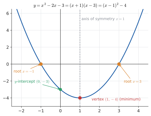
Read it carefully, because every label is a fact you can compute from the symbols:
-
\(a = 1 > 0\), so the parabola opens upwards and the vertex is a minimum.
-
The \(y\)-intercept is \(c = -3\) (set \(x = 0\)).
-
The roots are \(-1\) and \(3\), because \(x^2 - 2x - 3 = (x + 1)(x - 3)\).
-
The axis of symmetry is halfway between the roots, \(x = 1\), which agrees with \(-b/(2a) = -(-2)/2 = 1\).
-
The vertex is \((1, f(1)) = (1, 1 - 2 - 3) = (1, -4)\).
-
The discriminant is \((-2)^2 - 4(1)(-3) = 4 + 12 = 16 > 0\): two roots, as seen.
8.3. One object, four representations
The project specification behind this book singles out the quadratic as the example of something that is simultaneously an expression, a function, a curve, a set of roots, a computation and a model. Fluency means moving between these views without friction, so it is worth making each translation explicit before learning any solution method.
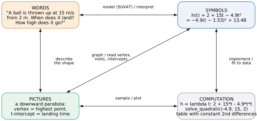
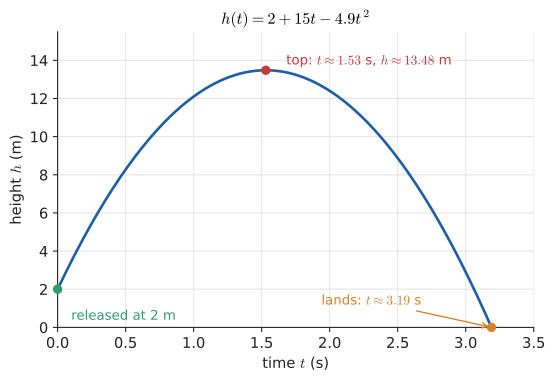
Words → symbols. "Thrown up at 15 m/s from 2 m" becomes \(h(t) = 2 + 15t - 4.9t^2\) via the SUVAT equation. Each coefficient has a physical meaning: \(c = 2\) is the starting height, \(b = 15\) the starting speed, \(a = -4.9 = -\tfrac12 g\) half the acceleration. Negative \(a\): the parabola opens downwards, so there is a maximum height. The words predicted the shape before you drew anything. Try it: Explore the thrown ball’s parabola.
Symbols → pictures. Different symbolic forms reveal different features of the graph. Standard form \(ax^2 + bx + c\) shows the \(y\)-intercept \(c\). Factored form \(a(x - r_1)(x - r_2)\) shows the roots. Vertex form \(a(x - h)^2 + k\) shows the vertex \((h, k)\) (Section 8.8). For the ball, vertex form is approximately \(h(t) = -4.9(t - 1.53)^2 + 13.48\): the peak at \(t \approx 1.53\) s, height \(\approx 13.48\) m, is visible without plotting a single point.
Pictures → words. "Symmetric about its peak" says: the ball takes as long to climb from the release height to the top as to fall back to that height. "Two intercepts, one of them at negative time" says: the equation has a root at negative \(t\) that the physics throws away (it is when the ball would have been at ground level, had its parabolic flight started earlier).
Symbols ↔ computation. A quadratic is a three-number object \((a, b, c)\) that a computer evaluates with two multiplications and two additions (Horner, Chapter 7). Going the other way, computation reveals a quadratic hiding in data: in a table of values at equally spaced inputs, the second differences are constant and equal to \(2a\) times the square of the spacing.
def f(x):
    return x**2 - 2*x - 3

xs = list(range(-1, 5))
ys = [f(x) for x in xs]
d1 = [b - a for a, b in zip(ys, ys[1:])]     # first differences
d2 = [b - a for a, b in zip(d1, d1[1:])]     # second differences
print("x :", xs)
print("y :", ys)
print("d1:", d1)
print("d2:", d2)
Try it: See the differences table live.
x : [-1, 0, 1, 2, 3, 4]
y : [0, -3, -4, -3, 0, 5]
d1: [-3, -1, 1, 3, 5]
d2: [2, 2, 2, 2]
Linear functions have constant first differences (constant slope, Chapter 5). Quadratics have constant second differences: the slope itself changes at a constant rate. That is exactly what constant acceleration means for the ball: velocity changes steadily, so position is quadratic. In Chapter 17 you will see this as "the second derivative of a quadratic is the constant \(2a\)".
|
Four views at once
Three sliders for \(a\), \(b\), \(c\). Four synchronised panels: the equation in standard, vertex and factored form (factored form greys out when there are no real roots); the parabola with vertex, axis and roots marked; a table of values with first and second differences; and a short sentence in words ("opens downward, maximum 13.48 at t = 1.53, two real roots"). Drag the graph’s vertex directly and watch the coefficients change. |
8.4. Method 1: solving by factoring
8.4.1. The problem
Solve \(x^2 - 5x + 6 = 0\).
8.4.2. Intuition and why it works
If you can write the quadratic as a product of two linear factors, the zero-product property (Chapter 7) finishes the job: a product is zero exactly when one of its factors is zero. For a monic quadratic \(x^2 + bx + c\), expanding \((x + m)(x + n) = x^2 + (m + n)x + mn\) shows you need two numbers with sum \(b\) and product \(c\).
Input: a quadratic equation.
Steps:
-
Rearrange to standard form \(ax^2 + bx + c = 0\) (everything on one side, zero on the other).
-
Remove any common factor.
-
Factor: for \(a = 1\), find \(m, n\) with \(m + n = b\), \(mn = c\); for \(a \neq 1\), use the \(ac\) method (Chapter 7).
-
Set each factor equal to zero and solve the resulting linear equations.
-
Check each root in the original equation.
Output: the roots, or "does not factor over the integers" (then switch method).
8.4.3. Worked examples
(a) \(x^2 - 5x + 6 = 0\). Need sum \(-5\), product \(6\): \(-2\) and \(-3\).
Check: \(4 - 10 + 6 = 0\) ✓, \(9 - 15 + 6 = 0\) ✓.
(b) \(2x^2 + x = 6\).
(c) The break-even problem: \(-2q^2 + 120q - 1000 = 0\).
The company breaks even at 1,000 and 5,000 units (\(q\) counts hundreds).
(d) \(x^2 = 7x\). Do not divide by \(x\):
|
Factoring pitfalls
|
When to choose it. When the coefficients are small integers and you can see the factor pair within a few seconds. A quick test: a quadratic with integer coefficients factors over the integers exactly when its discriminant \(b^2 - 4ac\) is a perfect square (\(0, 1, 4, 9, 16, \ldots\)). For \(x^2 - 5x + 6\), \(\Delta = 25 - 24 = 1 = 1^2\): factor it.
8.5. Method 2: completing the square
8.5.1. The problem
Solve \(x^2 + 6x - 7 = 0\), but pretend you cannot see the factorisation. More to the point: find a method that works for every quadratic, including \(x^2 - 2x - 1 = 0\), which does not factor nicely.
8.5.2. Intuition: equations that are easy
Some quadratics are trivially easy. \(x^2 = 16\) gives \(x = \pm 4\). Equally easy is
What makes these easy is that \(x\) appears only once, inside a square, so you can undo the square with a square root and then undo the addition. The general quadratic \(x^2 + 6x - 7\) has \(x\) in two places (\(x^2\) and \(6x\)). Completing the square merges those two appearances into one.
8.5.3. Why it works: literally completing a square
Think of \(x^2 + 6x\) as an area: an \(x\)-by-\(x\) square plus a rectangle \(6\) by \(x\). Cut the rectangle into two halves, each \(3\) by \(x\), and attach one to the right side of the square and the other to the top. You now have an almost-square shape of side \(x + 3\), missing a \(3\)-by-\(3\) corner.
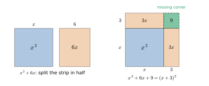
Add that corner, area \(3^2 = 9\), and you have completed the square:
In general, half the coefficient of \(x\), squared, is the missing corner:
(Expand the right side to check: \(x^2 + 2\cdot\tfrac{p}{2}x + \tfrac{p^2}{4} = x^2 + px + \tfrac{p^2}{4}\).) This is the perfect-square identity \((a + b)^2 = a^2 + 2ab + b^2\) from Chapter 7, read backwards.
To keep an equation balanced, whatever you add to one side you must add to the other.
Input: \(a, b, c\) with \(a \neq 0\).
Steps:
-
If \(a \neq 1\), divide every term by \(a\). Now the equation is \(x^2 + px + q = 0\).
-
Move the constant to the right: \(x^2 + px = -q\).
-
Add \((p/2)^2\) to both sides.
-
Rewrite the left side as \((x + p/2)^2\); simplify the right side to a single number \(R\).
-
If \(R < 0\): no real solutions (a square cannot be negative); stop.
-
Take square roots of both sides, remembering \(\pm\): \(x + p/2 = \pm\sqrt{R}\).
-
Subtract \(p/2\): \(x = -p/2 \pm \sqrt{R}\).
Output: the real roots (two if \(R > 0\), one if \(R = 0\)).
8.5.4. Worked example 1: \(x^2 + 6x - 7 = 0\)
Cross-check by factoring: \(x^2 + 6x - 7 = (x + 7)(x - 1)\) ✓.
8.5.5. Worked example 2: leading coefficient not 1, irrational roots
Solve \(2x^2 - 8x + 3 = 0\).
Numerically \(\sqrt{10}/2 \approx 1.5811\), so \(x \approx 3.5811\) or \(x \approx 0.4189\). Check the first: \(2(3.5811)^2 - 8(3.5811) + 3 \approx 25.649 - 28.649 + 3 = 0.000\) ✓.
8.5.6. Worked example 3: no real roots
Solve \(x^2 - 2x + 3 = 0\). Try it: See the roots 1 ± i√2.
A real number squared is never negative, so there are no real solutions. Geometrically, the parabola \(y = (x - 1)^2 + 2\) has its lowest point at height 2 and never reaches the axis. (In Chapter 15 you will allow \(\sqrt{-2} = i\sqrt 2\), and this equation gets the two roots \(1 \pm i\sqrt{2}\).)
8.5.7. Where you’d use this
Completing the square turns "find the best value" into "read off the vertex", because \(a(x - h)^2 + k\) is smallest (for \(a > 0\)) when the square is zero.
-
Statistics: why the mean? Given data \(2, 4, 9\), which single number \(c\) is "closest" to all of them, in the sense of making the sum of squared errors \(S(c) = (c - 2)^2 + (c - 4)^2 + (c - 9)^2\) smallest? Expanding, \(S(c) = 3c^2 - 30c + 101 = 3(c - 5)^2 + 26\). The minimum is at \(c = 5\), which is exactly the mean, with \(S = 26\) (try \(c = 4\): \(S = 29\)). The same algebra with \(n\) data points shows that the mean always minimises squared error, which is why least-squares fitting (Chapter 31) and the "mean squared error" loss in machine learning lead back to averages.
-
Optimisation by hand. The fence and café-revenue problems in Section 8.14 are vertex-reading problems; completing the square is how you find a maximum without calculus.
|
Completing-the-square slips
|
Why bother, when there is a formula? Three reasons. Completing the square is how the formula is derived (next section). It produces vertex form, which tells you the maximum or minimum of a quadratic (Section 8.8). And it generalises: you will complete the square again for circles (Chapter 10), in integrals (Chapter 19), and for the Gaussian distribution (Chapter 30).
|
Al-Khwarizmi’s square
The geometric picture above is essentially the one in Muhammad ibn Musa al-Khwarizmi’s The Compendious Book on Calculation by Completion and Balancing (Baghdad, around 820 CE). His worked problem was "a square and ten roots are equal to thirty-nine", i.e. \(x^2 + 10x = 39\); he split the ten into strips of five, completed the square with \(25\), got \(64 = 8^2\), and so \(x = 3\). (He ignored the negative root \(-13\); negative numbers were not yet accepted as answers.) The "completion" in his title is al-jabr, from which we get the word algebra; his own name gives us algorithm. Babylonian scribes solved the same kind of problem on clay tablets around 1800 BCE, using recipes that amount to the same steps. |
8.6. Method 3: the quadratic formula, derived
8.6.1. The problem
Completing the square works every time, but it means redoing the same steps for each new equation. As programmers know, when you find yourself repeating a procedure with different inputs, you write a function. The quadratic formula is completing the square done once, symbolically, for general \(a, b, c\).
8.6.2. Derivation, every step shown
Start from the general quadratic, with \(a \neq 0\):
Two steps deserve a comment.
-
Where the discriminant appears. After completing the square, the right-hand side is \((b^2 - 4ac)/(4a^2)\). The denominator \(4a^2\) is always positive, so the sign of the right-hand side is the sign of \(b^2 - 4ac\). A square cannot equal a negative number, so if \(b^2 - 4ac < 0\) the derivation stops: no real roots. The discriminant is not an arbitrary extra rule; it is the quantity whose square root you need.
-
The \(|a|\) subtlety. \(\sqrt{4a^2} = 2|a|\), not \(2a\) (if \(a = -3\), \(\sqrt{36} = 6 = 2|a|\)). But since we are taking \(\pm\) anyway, \(\pm\frac{\sqrt{\Delta}}{2|a|}\) and \(\pm\frac{\sqrt{\Delta}}{2a}\) describe the same pair of numbers.
|
Quadratic formula
The solutions of \(ax^2 + bx + c = 0\) (\(a \neq 0\)) are
\[x = \frac{-b \pm \sqrt{b^2 - 4ac}}{2a} .\]
Read it as "the axis of symmetry \(-b/(2a)\), plus or minus a half-width \(\sqrt{\Delta}/(2a)\)". The two roots are symmetric about the vertex. |
That reading is worth pausing on. The formula says the roots are
which is exactly what the picture of the parabola shows: two roots, mirror images about the vertical line through the vertex.
Input: a quadratic equation.
Steps:
-
Rearrange to \(ax^2 + bx + c = 0\) and write down \(a\), \(b\), \(c\) with their signs.
-
Compute the discriminant \(\Delta = b^2 - 4ac\).
-
If \(\Delta < 0\): no real roots (two complex roots, Chapter 15). Stop.
-
If \(\Delta = 0\): one repeated root \(x = -b/(2a)\). Stop.
-
Otherwise compute \(\sqrt{\Delta}\) and the two roots \(x = (-b \pm \sqrt\Delta)/(2a)\).
-
Simplify surds if an exact answer is wanted; otherwise round only at the end.
-
Check (substitute, or use Vieta’s formulas, Section 8.12).
Output: zero, one or two real roots.
8.6.3. Worked example: \(3x^2 - 5x - 1 = 0\)
\(a = 3\), \(b = -5\), \(c = -1\).
With \(\sqrt{37} \approx 6.0828\): \(x \approx \frac{11.0828}{6} \approx 1.8471\) or \(x \approx \frac{-1.0828}{6} \approx -0.1805\).
Check with Vieta (Section 8.12): sum of roots should be \(-b/a = 5/3 \approx 1.6667\); \(1.8471 + (-0.1805) = 1.6666\) ✓. Product should be \(c/a = -1/3\); \(1.8471 \times (-0.1805) \approx -0.3334\) ✓.
8.6.4. Worked example: the ball lands
\(-4.9t^2 + 15t + 2 = 0\): \(a = -4.9\), \(b = 15\), \(c = 2\).
The ball hits the ground after about \(3.19\) s. The negative root is discarded: the model only applies after release. (Discarding roots for physical reasons is normal and is part of the modelling step, not a defect of the mathematics.)
8.6.5. Where you’d use this
The formula is for the quadratics that do not factor nicely, which is nearly all of them in practice.
-
Road safety. A driver needs 0.7 s to react, then brakes at \(6\ \text{m/s}^2\). At speed \(u\) m/s the stopping distance is \(0.7u + \frac{u^2}{12}\) (thinking distance plus braking distance \(u^2/(2 \times 6)\)). What is the fastest speed from which the car can stop within 40 m? Multiply \(0.7u + \frac{u^2}{12} = 40\) by 12: \(u^2 + 8.4u - 480 = 0\), so \(u = \frac{-8.4 + \sqrt{8.4^2 + 1920}}{2} = \frac{-8.4 + 44.62}{2} \approx 18.1\) m/s, about 65 km/h. (The negative root is discarded.)
-
Finance: rate of return. You invest $1000 and receive $600 after one year and $600 after two. The yearly return \(r\) that makes this fair satisfies \(1000 = \frac{600}{g} + \frac{600}{g^2}\) with \(g = 1 + r\). Multiplying by \(g^2\): \(1000g^2 - 600g - 600 = 0\), so \(g = \frac{600 + \sqrt{600^2 + 4 \cdot 1000 \cdot 600}}{2000} \approx 1.1307\). The internal rate of return is about 13.1% a year. With more years of payments the equation becomes a higher-degree polynomial, and spreadsheets solve it numerically.
-
Computing. Every ray tracer and many collision detectors solve this formula millions of times per second (Section 8.15), which is why its numerical behaviour (Section 8.11) matters.
|
Quadratic-formula slips
|
|
Did anyone discover "the" formula?
No single person. The Indian mathematician Brahmagupta (628 CE) stated a rule in words equivalent to the formula for one root, and Sridhara (around 900 CE) gave a version that is close to the modern form. The compact symbolic formula needed symbolic algebra itself, which arrived with Viète (1590s) and Descartes (1637). Before that every rule was a recipe written in prose, which is one reason a "procedure" box is such a natural way to present it: that is how it was first written down. |
8.7. The discriminant: how many roots, before you find them
8.7.1. The problem
Sometimes you do not need the roots, only to know whether they exist. Does a ray hit a sphere (Section 8.15)? Does a ball thrown at a given speed ever reach a given height? Is a trinomial factorable over the integers? All three are answered by the sign (or the squareness) of one number.
8.7.2. Why it works
The derivation showed
The left side is a square, hence \(\ge 0\). So:
-
\(\Delta > 0\): the right side is positive and has two square roots, \(\pm\sqrt{\Delta}/(2a)\): two distinct real roots.
-
\(\Delta = 0\): the right side is zero, whose only square root is \(0\): one repeated root \(x = -b/(2a)\), a root of multiplicity 2 (Chapter 7). The quadratic is a perfect square \(a(x + b/2a)^2\).
-
\(\Delta < 0\): the right side is negative and no real number squares to it: no real roots (two complex-conjugate roots).
Graphically, the discriminant measures how far the vertex is from the \(x\)-axis, relative to how the parabola opens. The vertex height is \(k = -\Delta/(4a)\) (we prove this in Section 8.8). For an upward parabola (\(a > 0\)), \(\Delta > 0\) means \(k < 0\): the minimum is below the axis, so the curve must cross it twice.
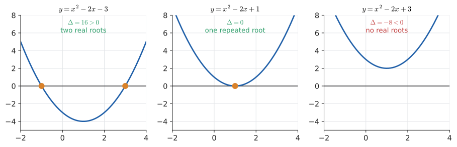
8.7.3. Worked example
How many real roots does each have?
| Equation | \(\Delta = b^2 - 4ac\) | Conclusion |
|---|---|---|
\(x^2 - 2x - 3 = 0\) |
\(4 + 12 = 16\) |
two; and \(16 = 4^2\), so it factors: \((x+1)(x-3)\) |
\(4x^2 - 12x + 9 = 0\) |
\(144 - 144 = 0\) |
one repeated: \(x = 12/8 = 3/2\); \((2x - 3)^2\) |
\(x^2 - 2x + 3 = 0\) |
\(4 - 12 = -8\) |
none (real) |
\(x^2 - 2x - 1 = 0\) |
\(4 + 4 = 8\) |
two irrational: \(1 \pm \sqrt 2\) |
Does the ball reach 15 m? Solve \(2 + 15t - 4.9t^2 = 15\), i.e. \(-4.9t^2 + 15t - 13 = 0\). \(\Delta = 225 - 4(-4.9)(-13) = 225 - 254.8 = -29.8 < 0\). No: it never gets that high (consistent with the peak of 13.48 m). Does it reach 10 m? \(-4.9t^2 + 15t - 8 = 0\) has \(\Delta = 225 - 156.8 = 68.2 > 0\): yes, twice, once going up and once coming down.
8.7.4. Where you’d use this
The discriminant answers yes/no questions ("does it ever happen?") without solving anything.
-
Everyday geometry. Can a rectangle with perimeter 20 m have area 30 m²? Sides \(x\) and \(10 - x\) give \(x(10 - x) = 30\), i.e. \(x^2 - 10x + 30 = 0\), with \(\Delta = 100 - 120 = -20 < 0\). No: the largest area with that perimeter is the 5 by 5 square, 25 m².
-
Engineering: springs and dampers. A car’s suspension, a door closer and a measuring instrument’s needle all behave like a mass \(m\) on a spring of stiffness \(k\) with damping \(c\). Their motion is governed by the roots of \(ms^2 + cs + k = 0\), and the sign of \(\Delta = c^2 - 4mk\) decides the character. \(\Delta < 0\): it overshoots and oscillates (underdamped). \(\Delta > 0\): it creeps back slowly (overdamped). \(\Delta = 0\): it returns as fast as possible without overshooting (critically damped). For \(m = 1\) kg and \(k = 100\) N/m, critical damping needs \(c^2 = 400\), i.e. \(c = 20\) N·s/m. Engineers tune door closers and instrument needles to sit near that value.
-
Computing. A ray misses a sphere exactly when the discriminant of its intersection quadratic is negative, so a renderer can reject most rays with one multiply-and-compare and never take a square root (Section 8.15).
|
Factorability test
A quadratic \(ax^2 + bx + c\) with integer coefficients factors into linear factors with integer (or rational) coefficients if and only if its discriminant is a perfect square. Reason: the roots \((-b \pm \sqrt\Delta)/(2a)\) are rational exactly when \(\sqrt\Delta\) is. |
|
Discriminant explorer
Fix \(a\) and \(b\); slide \(c\). Watch the parabola rise, the two roots slide together, merge at \(\Delta = 0\), and vanish. A second panel plots the roots in the complex plane: as they leave the real axis they become a symmetric pair \(p \pm qi\) moving vertically, preparing the ground for Chapter 15. |
8.8. Three forms, and the graph of a quadratic
8.8.1. The problem
Find the maximum height of the ball and when it occurs; find the best fence. These are questions about the vertex, not the roots. Each of the three standard ways of writing a quadratic answers a different question directly:
| Form | Formula | Reveals |
|---|---|---|
Standard |
\(y = ax^2 + bx + c\) |
\(y\)-intercept \(c\); coefficients for the formula and discriminant |
Factored (intercept) |
\(y = a(x - r_1)(x - r_2)\) |
roots \(r_1, r_2\) |
Vertex |
\(y = a(x - h)^2 + k\) |
vertex \((h, k)\), axis \(x = h\), max/min value \(k\) |
In all three, \(a\) is the same number and has the same meaning: direction (sign) and steepness (size).
8.8.2. Transformations of \(y = x^2\)
Vertex form is easiest to understand as a sequence of moves applied to the basic parabola \(y = x^2\), whose vertex is the origin.
-
\(y = x^2 + k\): shift up by \(k\) (down if \(k < 0\)).
-
\(y = (x - h)^2\): shift right by \(h\). (The minus sign surprises people. The new curve reaches height 0 when \(x - h = 0\), i.e. at \(x = h\), so the vertex has moved to \(x = h\).)
-
\(y = ax^2\): stretch vertically by factor \(a\); \(|a| > 1\) is narrower, \(|a| < 1\) wider; \(a < 0\) also reflects in the \(x\)-axis.
Combining them: \(y = a(x - h)^2 + k\) is \(y = x^2\) stretched by \(a\), then moved so that its vertex is at \((h, k)\).
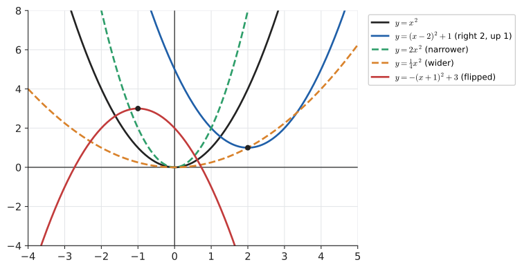
These rules are not special to parabolas. Replacing \(x\) by \(x - h\) shifts any graph right by \(h\), and multiplying by \(a\) stretches any graph vertically. You will reuse this exact toolkit for every function family in Chapter 11.
8.8.3. Converting between forms
Standard → vertex: complete the square (keeping the equation as a function, so we add and subtract rather than adding to both sides).
Input: \(y = ax^2 + bx + c\).
Steps:
-
Factor \(a\) out of the first two terms: \(y = a\left(x^2 + \frac{b}{a}x\right) + c\).
-
Inside the bracket, add and subtract \(\left(\frac{b}{2a}\right)^2\).
-
Write the first three terms inside as a square; move the subtracted term out of the bracket (multiplying it by \(a\)).
-
Simplify the constant.
Output: \(y = a(x - h)^2 + k\) with \(h = -\dfrac{b}{2a}\) and \(k = c - \dfrac{b^2}{4a}\).
Worked example. Write \(y = 2x^2 - 12x + 13\) in vertex form.
Vertex \((3, -5)\), a minimum because \(a = 2 > 0\). The minimum value of \(2x^2 - 12x + 13\) is \(-5\), attained at \(x = 3\).
The general vertex. Doing the same symbolically:
So \(h = -b/(2a)\) and \(k = -\Delta/(4a)\), which is the fact we used in Section 8.7.
Vertex → standard: expand. \(2(x - 3)^2 - 5 = 2(x^2 - 6x + 9) - 5 = 2x^2 - 12x + 13\).
Standard → factored: find the roots. By any method; then \(ax^2 + bx + c = a(x - r_1)(x - r_2)\). For \(2x^2 - 12x + 13\): \(2(x - 3)^2 = 5\) gives \(x = 3 \pm \sqrt{5/2}\), so \(y = 2\left(x - 3 - \sqrt{5/2}\right)\left(x - 3 + \sqrt{5/2}\right)\). Do not forget the leading \(a\): the factored form of \(2x^2 - 12x + 13\) is not \((x - r_1)(x - r_2)\), which has leading coefficient 1.
Factored → vertex: average the roots. The vertex is midway between the roots: \(h = (r_1 + r_2)/2\); then \(k = f(h)\). For \(y = (x + 1)(x - 3)\): \(h = (-1 + 3)/2 = 1\), \(k = (2)(-2) = -4\). Vertex \((1, -4)\), matching the anatomy diagram.
8.8.4. Sketching a parabola by hand
Steps:
-
Sign of \(a\): cup (\(a > 0\)) or cap (\(a < 0\)).
-
\(y\)-intercept \((0, c)\).
-
Vertex \(h = -b/(2a)\), \(k = f(h)\); draw the axis \(x = h\).
-
Discriminant: if \(\Delta \ge 0\), find the roots and mark them.
-
Reflect the \(y\)-intercept in the axis to get a free extra point \((2h, c)\).
-
Draw a smooth symmetric curve through the points.
For the ball: cap; intercept \((0, 2)\); vertex at \(t = -15/(2 \cdot (-4.9)) = 15/9.8 \approx 1.531\), \(h(1.531) = 2 + 225/19.6 \approx 13.48\); roots \(\approx -0.128\) and \(\approx 3.189\); mirror point \((3.061, 2)\).
8.9. Method 4 and 5: graphing and numerical root finding
8.9.1. Graphing
Plot \(y = ax^2 + bx + c\) and read off where it crosses the axis. On paper this gives one or two significant figures; with graphing software or a zoomable plot, more. Its real value is not precision but understanding: a graph shows at a glance how many roots there are, roughly where, and whether the answer from a formula is plausible. Graphing is also the natural method when the "quadratic" is buried in a more complicated equation, such as \(x^2 = 2^x\), where you might first want to know how many solutions to look for (there are three).
8.9.2. Numerical root finding
A numerical method does not produce a formula; it produces a sequence of better and better approximations. For a quadratic this is usually unnecessary, because the formula exists. But understanding the numerical approach here, where you can check the answer exactly, prepares you for equations that have no formula: polynomials of degree 5 and above, equations mixing polynomials with \(e^x\) or \(\sin x\), and the equations inside every physics engine.
Bisection is the simplest. If a continuous function is negative at one point and positive at another, it must cross zero somewhere between (the intermediate value theorem, Chapter 16). Repeatedly halve the interval, keeping the half where the sign change is.
Input: continuous \(f\), an interval \(\lbrack lo, hi]\) with \(f(lo)\) and \(f(hi)\) of opposite signs, a tolerance \(\varepsilon\).
Steps:
-
Compute the midpoint \(m = (lo + hi)/2\).
-
If \(f(m)\) has the same sign as \(f(lo)\), set \(lo \leftarrow m\); otherwise set \(hi \leftarrow m\).
-
Repeat until \(hi - lo < \varepsilon\).
Output: \(m\), within \(\varepsilon\) of a root. Each step halves the uncertainty, gaining one binary digit of accuracy.
def bisect(f, lo, hi, tol=1e-12):
    """Find a root of f in [lo, hi], assuming f(lo) and f(hi) differ in sign."""
    flo = f(lo)
    steps = 0
    while hi - lo > tol:
        mid = (lo + hi) / 2
        fmid = f(mid)
        if (fmid > 0) == (flo > 0):     # same sign as left end: root is right
            lo, flo = mid, fmid
        else:
            hi = mid
        steps += 1
    return (lo + hi) / 2, steps

root, steps = bisect(lambda x: x*x - 2*x - 1, 2, 3)
print(root, steps)       # exact answer: 1 + sqrt(2) = 2.41421356237...
Try it: Run these 40 halvings.
2.414213562372879 40
Forty halvings to get twelve decimal places: steady but slow.
Newton’s method is much faster. Starting from a guess \(x_0\), it repeatedly slides down the tangent line to where the tangent meets the axis:
where \(f'(x)\) is the derivative, the slope of the tangent, which for \(f(x) = ax^2 + bx + c\) is \(2ax + b\). You will derive this properly in Chapter 17 and study Newton’s method, and how it can fail, in Chapter 18. For a preview, take \(f(x) = x^2 - 2\) (root \(\sqrt 2\)) and \(x_0 = 1\): the iteration is \(x_{n+1} = x_n - (x_n^2 - 2)/(2x_n)\), giving \(1 \to 1.5 \to 1.41\overline{6} \to 1.4142157 \to 1.41421356237469\). The number of correct digits roughly doubles each step: four steps where bisection would need about forty.
|
Bisection versus Newton
Plot a quadratic and run bisection and Newton side by side, one step per click. Bisection shows a shrinking bracket; Newton shows tangent lines. Choose \(x_0\) exactly at the vertex and watch Newton fail (horizontal tangent, division by zero); start Newton on \(x^2 + 1\) and watch it wander chaotically, because there is no real root to find. |
8.10. Choosing a method
You now have five ways to solve a quadratic. They are not interchangeable: each has a sweet spot.
A quadratic such as \(x^2 - 5x + 6 = 0\) practically begs to be factored: two numbers with sum 5 and product 6 jump out, and \((x - 2)(x - 3) = 0\) is done in seconds with exact answers. Using Newton’s method there would be rather silly: you would get \(2.0000000000\) after several iterations of arithmetic, and you would still have to run it again from a different starting point to find the other root. Conversely, trying to factor \(3x^2 - 5x - 1\) wastes time hunting for integer pairs that do not exist.
| Method | Use when | Avoid when |
|---|---|---|
Factoring |
small integer coefficients; \(\Delta\) is a perfect square; you want exact roots fast |
roots are irrational or the coefficients are large or decimal |
Completing the square |
you need vertex form (max/min); \(a = 1\) and \(b\) even; deriving things |
messy fractions would appear and you only want roots |
Quadratic formula |
any quadratic, by hand, when factoring is not obvious; exact surd answers |
on a computer when \(b^2 \gg 4ac\), unless you use the stable variant |
Graphing |
you want to understand: how many roots, roughly where, sanity checks |
you need several significant figures |
Numerical (bisection, Newton) |
the quadratic is part of a bigger non-polynomial equation; high-degree polynomials; inside an iterative algorithm |
a closed form exists and you only need this one quadratic solved |
Steps:
-
Put it in standard form. If \(b = 0\) (\(ax^2 + c = 0\)), solve directly: \(x^2 = -c/a\). If \(c = 0\), factor out \(x\).
-
Compute \(\Delta\). If \(\Delta < 0\) and you only want real roots, stop.
-
If \(\Delta\) is a perfect square and the coefficients are small, factor.
-
If you also need the vertex, complete the square.
-
Otherwise use the quadratic formula (by hand), or the numerically stable formula (on a computer).
-
Sketch or estimate to sanity-check the answer.
Worked example of choosing. Which method for each?
-
\(x^2 - 49 = 0\): \(b = 0\), so \(x = \pm 7\) directly. (Difference of squares, if you prefer.)
-
\(x^2 + 8x + 11 = 0\): \(\Delta = 64 - 44 = 20\), not a square, but \(b\) is even and \(a = 1\): completing the square is quick: \((x + 4)^2 = 5\), \(x = -4 \pm \sqrt5\).
-
\(0.37x^2 - 1.92x + 0.5 = 0\): decimals, so formula (or calculator): \(\Delta = 3.6864 - 0.74 = 2.9464\), \(x = (1.92 \pm 1.7165)/0.74\), so \(x \approx 4.914\) or \(x \approx 0.2750\).
-
\(x^2 = \cos x\): not a quadratic at all; graph to see there are two solutions (near \(\pm 0.82\)), then Newton.
8.11. When the formula fails: catastrophic cancellation
8.11.1. The problem
The quadratic formula is exact. Floating-point arithmetic is not. Solve Try it: See the 25% error.
on a computer using the formula exactly as written:
import math

def naive_roots(a, b, c):
    d = math.sqrt(b * b - 4 * a * c)
    return (-b + d) / (2 * a), (-b - d) / (2 * a)

print(naive_roots(1.0, -1e8, 1.0))
(100000000.0, 7.450580596923828e-09)
The roots multiply to \(c/a = 1\) (Vieta), so if one is \(10^8\) the other must be \(10^{-8}\) (to about 16 digits: the exact small root is \(1.0000000000000000 \times 10^{-8}\)). The computer reports \(7.45 \times 10^{-9}\): an error of 25%, from a formula you just derived with complete rigour. Nothing is wrong with the algebra. Something is wrong with how the computer carried it out.
8.11.2. Why it happens
A double-precision float carries about 16 significant decimal digits (Chapter 32). Here \(b^2 = 10^{16}\) and \(4ac = 4\). Then
That number needs 18 significant digits, but doubles near \(10^8\) are spaced \(2^{-26} \approx 1.49 \times 10^{-8}\) apart, so the nearest one the computer can store is \(10^8 - 1.49 \times 10^{-8}\). The small root is computed as
the difference of two nearly equal numbers. Their first 16 digits agree and cancel, leaving only the last one or two digits, which are mostly rounding error: the computer gets \((1.49 \times 10^{-8})/2 \approx 7.45 \times 10^{-9}\), exactly the wrong answer printed above. This is catastrophic cancellation: subtraction of nearly equal approximate quantities destroys relative accuracy. The large root, \((-b + \sqrt\Delta)/(2a)\), adds two numbers of the same sign and is perfectly accurate.
|
Catastrophic cancellation
Catastrophic cancellation is the loss of significant digits when two nearly equal floating-point numbers are subtracted. The subtraction itself is exact; the problem is that the inputs' small rounding errors become large relative to the small result. The cure is almost always algebraic: rewrite the expression so the subtraction never happens. |
8.11.3. A by-hand version
You can see the effect without a computer by pretending your calculator keeps only 4 significant digits. Solve \(x^2 + 62.10x + 1 = 0\) (true roots \(\approx -0.01611\) and \(\approx -62.08\)): Try it: The 4-digit calculator.
The answer \(-0.02000\) is 24% too large in magnitude. The other root, \((-62.10 - 62.06)/2 = -124.16/2 \to -124.2/2 = -62.10\), is off only in its last digit (true value \(-62.08\)).
8.11.4. The fix: compute the safe root first, then use Vieta
The product of the roots is \(x_1 x_2 = c/a\) (Section 8.12). So compute the root that involves no cancellation, and get the other from the product. Concretely, choose the sign in front of the square root to match the sign of \(b\), so that \(b\) and \(\operatorname{sign}(b)\sqrt\Delta\) add rather than cancel:
Here \(\operatorname{sign}(b)\) is \(+1\) if \(b \ge 0\) and \(-1\) if \(b < 0\). Why is \(c/q\) a root? Multiply the two roots from the textbook formula: \(\frac{-b + \sqrt\Delta}{2a}\cdot\frac{-b - \sqrt\Delta}{2a} = \frac{b^2 - \Delta}{4a^2} = \frac{4ac}{4a^2} = \frac{c}{a}\). So if \(x_1 = q/a\) is one root, the other is \(\frac{c/a}{q/a} = \frac{c}{q}\).
In the 4-digit example: \(62.10 + 62.06 = 124.16 \to 124.2\), so \(q = -62.10\), \(x_2 = q/a = -62.10\) and \(x_1 = c/q = 1/(-62.10) = -0.01610\). The true value is \(-0.016107\ldots\), so the small root is now off by at most one unit in the fourth digit, instead of 24%.
import math

def stable_roots(a, b, c):
    d = math.sqrt(b * b - 4 * a * c)
    q = -(b + math.copysign(d, b)) / 2   # b and +-d have the same sign: no cancellation
    return q / a, c / q

print(stable_roots(1.0, -1e8, 1.0))
(100000000.0, 1e-08)
math.copysign(d, b) returns \(d\) with the sign of \(b\): exactly the \(\operatorname{sign}(b)\sqrt\Delta\) term.
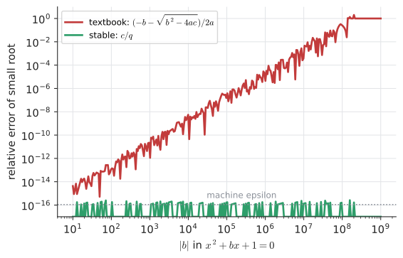
The plot tells the story: the textbook formula loses roughly two digits of accuracy for every factor of 10 in \(|b|\) (its relative error grows like \(b^2\) times the machine precision \(\approx 10^{-16}\), about 25% at \(|b| = 10^8\) and 100% from about \(1.34\times 10^8\)), while the stable version stays at full precision throughout. Try it: Slide b and watch digits go.
|
Formulas are not algorithms
A formula that is exactly correct in real-number arithmetic can be a poor algorithm in floating point. Warning signs: subtracting quantities that may be nearly equal; computing a small number as the difference of two large ones; adding terms of wildly different size. The quadratic formula has a second hazard: \(b^2\) can overflow (exceed \(\approx 1.8 \times 10^{308}\)) even when the roots are modest, so production solvers also rescale the coefficients. Even the discriminant itself suffers cancellation when \(b^2 \approx 4ac\) (nearly repeated roots); then the roots are genuinely sensitive to tiny changes in the coefficients, and no rewriting can fully fix that. This is the difference between an unstable algorithm (fixable) and an ill-conditioned problem (not), a distinction developed in Chapter 32. |
|
How much precision do you lose?
Slide \(b\) from \(10\) to \(10^{10}\) in \(x^2 + bx + 1 = 0\). Show both formulas' results digit by digit, with correct digits in green and wrong digits in red, and the number of lost digits plotted against \(\log_{10}|b|\). Add a "precision" switch (16, 7, or 4 significant digits) to see the same collapse happen earlier in single precision and in the by-hand 4-digit model. Try it: How much precision do you lose? |
|
The quadratic formula in the wild
George Forsythe’s 1966 essay "How do you solve a quadratic equation?" used exactly this example to argue that numerical analysis is not optional knowledge for anyone who computes. William Kahan, the principal architect of the IEEE 754 floating-point standard, later wrote a careful paper on computing the discriminant itself accurately, using fused multiply–add instructions. The humble quadratic is the classic test case that numerical analysts use to teach the subject. |
8.12. Vieta’s formulas: what the coefficients know about the roots
8.12.1. The problem
The stable algorithm relied on "the roots multiply to \(c/a\)". Where does that come from, and what else is true?
8.12.2. Why it works
If \(r_1\) and \(r_2\) are the roots of \(ax^2 + bx + c\), the factor theorem says
Two polynomials are equal for every \(x\) only if their coefficients match, so
|
Vieta’s formulas
For \(ax^2 + bx + c = 0\) with roots \(r_1, r_2\) (real or complex, counted with multiplicity):
\[r_1 + r_2 = -\frac{b}{a}, \qquad r_1 r_2 = \frac{c}{a} .\]
For a monic quadratic \(x^2 + bx + c\): the roots sum to \(-b\) and multiply to \(c\). This is exactly why factoring \(x^2 + bx + c\) means "find two numbers with sum \(b\) and product \(c\)" (the numbers are the negatives of the roots). |
8.12.3. Uses
-
Checking answers without substituting (as in the formula example above).
-
Building a quadratic from its roots. Roots \(3 \pm \sqrt2\): sum \(6\), product \(9 - 2 = 7\), so \(x^2 - 6x + 7 = 0\).
-
The other root for free. \(x = 2\) is a root of \(3x^2 - 4x - 4 = 0\); the product of roots is \(-4/3\), so the other root is \(-\tfrac{4}{3} \div 2 = -\tfrac{2}{3}\).
-
Stable computation, as in Section 8.11.
-
Symmetric expressions in the roots without finding them. For \(x^2 - 5x + 3 = 0\), \(r_1^2 + r_2^2 = (r_1 + r_2)^2 - 2r_1 r_2 = 25 - 6 = 19\).
|
Viète
François Viète (1540–1603), a French lawyer and royal cryptanalyst who broke Spanish ciphers for Henri IV, was among the first to use letters systematically for known quantities as well as unknowns, which is what made general formulas like these expressible at all. His relations extend to every degree: for a cubic \(x^3 + bx^2 + cx + d\) with roots \(r_1, r_2, r_3\), the roots sum to \(-b\), their pairwise products sum to \(c\), and their product is \(-d\). |
8.13. Quadratic inequalities
8.13.1. The problem
For which times is the ball above 10 m? For which production levels is the company profitable? These ask where a quadratic is positive (or negative), not where it is zero: inequalities such as \(-2q^2 + 120q - 1000 > 0\).
8.13.2. Intuition
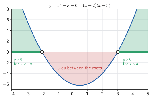
A parabola can only change sign where it crosses the axis, at its roots. Between consecutive roots its sign is constant. So: find the roots, then decide the sign on each interval. For an upward parabola (\(a > 0\)) with two roots, the quadratic is negative between the roots and positive outside them; for a downward one, the reverse.
Input: an inequality involving a quadratic.
Steps:
-
Rearrange to \(ax^2 + bx + c > 0\) (or \(<\), \(\ge\), \(\le\)): zero on one side.
-
Find the real roots (any method). If there are none, the quadratic has the sign of \(a\) everywhere: the solution is "all real \(x\)" or "no \(x\)".
-
Sketch the parabola (direction from \(a\); crossings at the roots), or make a sign table using test points.
-
Read off the intervals where the sign is as required. Include the roots for \(\ge\) or \(\le\); exclude them for \(>\) or \(<\).
Output: the solution set, as inequalities or interval notation.
8.13.3. Worked examples
(a) \(x^2 - x - 6 > 0\). Try it: Sign chart for x² − x − 6.
\(a = 1 > 0\), so the parabola is above the axis outside the roots: \(x < -2\) or \(x > 3\). A sign table confirms:
| Interval | \(x + 2\) | \(x - 3\) | product |
|---|---|---|---|
\(x < -2\) (test \(-3\)) |
\(-\) |
\(-\) |
\(+\) |
\(-2 < x < 3\) (test \(0\)) |
\(+\) |
\(-\) |
\(-\) |
\(x > 3\) (test \(4\)) |
\(+\) |
\(+\) |
\(+\) |
In interval notation the answer is \((-\infty, -2) \cup (3, \infty)\). Here round brackets mean the endpoint is excluded, square brackets would mean included, \(\infty\) is not a number but a marker for "no upper end", and \(\cup\) (union) means "or".
(b) \(-x^2 + 4x + 5 \ge 0\). Multiply by \(-1\) to make the leading coefficient positive, reversing the inequality: Try it: Sign chart for example (b).
(c) Profitable production: \(-2q^2 + 120q - 1000 > 0\) is \(q^2 - 60q + 500 < 0\) (divide by \(-2\), flip), i.e. \((q - 10)(q - 50) < 0\), so \(10 < q < 50\): between 1,000 and 5,000 units. Try it: Sign chart for the profit.
(d) The ball above 10 m: \(-4.9t^2 + 15t - 8 > 0\). Roots (formula, \(\Delta = 68.2\), \(\sqrt\Delta \approx 8.2583\)): \(t = (15 \mp 8.2583)/9.8 \approx 0.688\) and \(2.373\). Downward parabola, so positive between the roots: about \(0.69 < t < 2.37\) seconds, a window of \(\sqrt{\Delta}/|a| \approx 1.69\) s. Try it: When is the ball above 10 m?.
|
Inequality traps
|
Try it: Try a rational inequality.
8.14. Applications
8.14.1. Projectile motion
Every object moving under constant acceleration (and nothing else) has a position that is a quadratic function of time. That includes a thrown ball, a dropped phone, a braking car (constant deceleration), and a rocket in the short phase where thrust and gravity are roughly constant.
Worked example: maximum height. For \(h(t) = 2 + 15t - 4.9t^2\), the vertex is at
and the maximum height is
In SUVAT language you would have said: at the top the velocity is zero, \(v = u + at\) gives \(0 = 15 - 9.8t\), so \(t = 15/9.8\). Same answer, reached through physics instead of algebra, and a good illustration that the vertex of a quadratic is where its rate of change is zero, the idea that drives Chapter 18.
Braking distance. A car travelling at \(u\) m/s decelerates at \(d\) m/s². Its stopping distance is \(u^2/(2d)\): quadratic in speed. Doubling speed quadruples braking distance, which is why the UK Highway Code’s stopping distances grow so steeply.
8.14.2. Optimising area and revenue
Any quantity that is a product of two things, one increasing and one decreasing linearly in the same variable, is a downward quadratic and has a maximum at its vertex.
The fence. \(A(x) = x(100 - 2x) = -2x^2 + 100x\). Vertex at \(x = -100/(2 \cdot (-2)) = 25\). Area \(A(25) = 25 \times 50 = 1250\) m². Shortcut: the roots are \(0\) and \(50\), and the vertex is midway between them.
Revenue. A café’s simple demand model says it would sell 1000 coffees a week if they were free, and loses 20 weekly sales for every £1 on the price: demand \(q = 1000 - 20p\). Revenue is price times quantity:
Roots \(p = 0\) and \(p = 50\); vertex midway at \(p = 25\), with \(R(25) = 25 \times 500 = 12{,}500\), i.e. £12,500 a week. Raising the price beyond £25 loses more in volume than it gains in margin. (Real demand curves are not linear, but this is the first model economists draw, and the reasoning is the same with a better model plus calculus.)
The break-even company is at its best at the midpoint of its break-even volumes, \(q = 30\): \(P(30) = -1800 + 3600 - 1000 = 800\), i.e. £800,000 at 3,000 units.
8.14.3. The reflective property: dishes, headlights and telescopes
Every parabola has a special point, its focus. For \(y = \dfrac{x^2}{4f}\) the focus is at \((0, f)\). Every ray travelling parallel to the axis that hits the inside of the parabola reflects through the focus. Spin the parabola about its axis to get a paraboloid, and every parallel ray striking the dish converges at one point. Try it: Rays meeting at the focus.
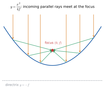
That is why:
-
Satellite dishes put the receiver at the focus: the faint parallel signal from a satellite 36,000 km away is concentrated there.
-
Reflecting telescopes (Newton’s design and every large modern telescope) use paraboloidal mirrors to bring starlight to a focus.
-
Headlights and torches run the reflection backwards: a bulb at the focus sends light out in a parallel beam.
-
Solar cookers and solar-thermal power plants concentrate sunlight on a pipe or pot at the focus.
Worked example: where to put the receiver. A dish is 60 cm across and 9 cm deep. Place its vertex at the origin, so its cross-section is \(y = x^2/(4f)\) and the rim is at \((30, 9)\): Try it: Place the receiver yourself.
The receiver sits 25 cm in front of the centre of the dish. The reason the property holds is a short calculation with distances: every point of the parabola is equally far from the focus and from a line called the directrix (\(y = -f\)); the proof uses tangent lines and is done in Chapter 10.
|
Whispering galleries and burning mirrors
A legend says Archimedes set fire to Roman ships at Syracuse (212 BCE) with "burning mirrors". Whether or not it happened (modern attempts have produced mixed results), Diocles' treatise On Burning Mirrors (around 190 BCE) contains the first known proof of the focal property of the parabola. The same geometry, applied to the ellipse, makes "whispering galleries" where a whisper at one focus is heard clearly at the other. |
8.15. Computer-science connection: ray–sphere intersection
8.15.1. The problem
A ray tracer makes images by firing a ray from the camera through each pixel and asking: what does this ray hit first? For a sphere, that question is a quadratic equation, solved millions of times per frame. This is perhaps the most-executed quadratic formula in the world.
8.15.2. Setting it up
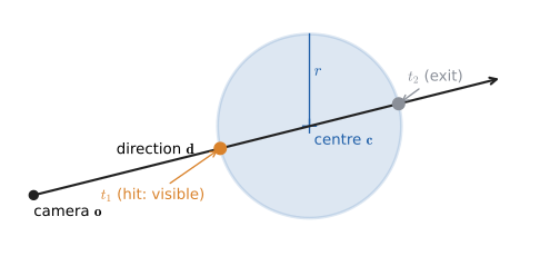
A ray starts at a point \(\mathbf{o}\) (the camera) and travels in direction \(\mathbf{d}\). Bold letters denote vectors, here just triples of numbers \((x, y, z)\) (Chapter 26). The points on the ray are
meaning: start at \(\mathbf{o}\) and move \(t\) units of \(\mathbf{d}\); component by component, \(p_x = o_x + t d_x\) and so on. The parameter \(t\) measures how far along the ray you are; smaller \(t\) is closer to the camera.
A sphere with centre \(\mathbf{c}\) and radius \(r\) is the set of points at distance \(r\) from \(\mathbf{c}\). Squared distance is computed by Pythagoras in 3D: for a vector \(\mathbf{v} = (v_x, v_y, v_z)\),
the dot product of \(\mathbf{v}\) with itself. More generally, \(\mathbf{u}\cdot\mathbf{v} = u_x v_x + u_y v_y + u_z v_z\); it distributes over addition just like ordinary multiplication.
8.15.3. Deriving the quadratic
The ray point \(\mathbf{p}(t)\) is on the sphere when its squared distance from the centre is \(r^2\). Write \(\mathbf{f} = \mathbf{o} - \mathbf{c}\) for the vector from the centre to the camera. Then \(\mathbf{p}(t) - \mathbf{c} = \mathbf{f} + t\mathbf{d}\), and
A quadratic in \(t\), and every piece of this chapter now has a geometric meaning:
-
\(\Delta < 0\): the ray misses the sphere. (This is the common case, and you can decide it without a square root.)
-
\(\Delta = 0\): the ray grazes the sphere tangentially.
-
\(\Delta > 0\): two intersections, \(t_1 < t_2\): entering and leaving. The visible surface is at the smallest positive \(t\).
-
\(t_1 < 0 < t_2\): the camera is inside the sphere.
-
Both negative: the sphere is behind the camera.
8.15.4. Worked example
Camera at \(\mathbf{o} = (0, 1, 0)\), looking along \(\mathbf{d} = (1, 0, 0)\); sphere centre \(\mathbf{c} = (5, 0, 0)\), radius \(r = 2\).
The visible point is at \(t \approx 3.268\): \(\mathbf{p} \approx (3.268, 1, 0)\). Check: its distance from the centre is \(\sqrt{(3.268 - 5)^2 + 1^2} = \sqrt{3.000 + 1} = 2\) ✓.
import math

def dot(u, v):
    return sum(ui * vi for ui, vi in zip(u, v))

def ray_sphere(origin, direction, centre, radius, eps=1e-9):
    """Smallest t > eps where origin + t*direction meets the sphere, or None."""
    f = [o - c for o, c in zip(origin, centre)]   # centre -> camera
    a = dot(direction, direction)
    b = 2 * dot(direction, f)
    c = dot(f, f) - radius * radius
    disc = b * b - 4 * a * c
    if disc < 0:
        return None                               # ray misses
    q = -0.5 * (b + math.copysign(math.sqrt(disc), b))   # stable formula
    if q == 0:
        return None                               # degenerate: grazing at origin
    t1, t2 = sorted((q / a, c / q))
    if t1 > eps:
        return t1                                 # first hit in front of camera
    if t2 > eps:
        return t2                                 # camera is inside the sphere
    return None                                   # sphere is behind the camera

print(ray_sphere((0, 1, 0), (1, 0, 0), (5, 0, 0), 2))   # hit
print(ray_sphere((0, 3, 0), (1, 0, 0), (5, 0, 0), 2))   # passes above: miss
print(ray_sphere((5, 0, 0), (1, 0, 0), (5, 0, 0), 2))   # from inside
3.267949192431123 None 2.0
The small eps guards against a classic ray-tracing bug, "shadow acne": a ray bounced off a surface, starting on that surface, finds a spurious intersection at \(t \approx 10^{-15}\) due to rounding, so the surface shadows itself. The stable formula matters here too, though not where you might guess. A small sphere far away is harmless: both formulas agree to about 16 digits. The textbook formula loses digits when \(c\) is tiny compared with \(b^2\), which happens when the ray starts very close to the surface of a large sphere (a shadow or reflection ray leaving a big floor or planet). Then the near root comes from cancellation, which is exactly the shadow-acne situation above.
|
A one-sphere ray tracer
A 200 by 200 pixel canvas. For each pixel, fire a ray and colour it by the discriminant: black for \(\Delta < 0\), and shaded by \(t_1\) (near is bright) otherwise. Move the camera into the sphere and watch the \(t_1 < 0 < t_2\) case take over. Then toggle "textbook formula" and push the sphere far away to see cancellation noise appear at the edges. |
8.16. Interactive tools
Browser tools on the companion website that go with this chapter. Each example link in the chapter opens one of them with that example already set up.
8.17. Exercises
-
(Recognition) For \(5 - 3x^2 + 2x = 0\), identify \(a\), \(b\), \(c\) and compute the discriminant. How many real roots?
-
(Recognition) Without solving, state the vertex, the axis of symmetry and whether the vertex is a maximum or minimum: (a) \(y = -3(x + 2)^2 + 7\) (b) \(y = (x - 4)(x + 6)\).
-
(Application) Solve by factoring: (a) \(x^2 + x - 20 = 0\) (b) \(3x^2 - 10x - 8 = 0\) (c) \(4x^2 = 9\).
-
(Application) Solve by completing the square, giving exact answers: (a) \(x^2 - 8x + 3 = 0\) (b) \(3x^2 + 12x - 1 = 0\).
-
(Application) Solve with the quadratic formula, giving exact and 4-significant-figure answers: \(2x^2 + 3x - 7 = 0\).
-
(Application) Write \(y = -x^2 + 6x - 5\) in vertex form and in factored form, and sketch it.
-
(Application) Solve \(2x^2 - 5x - 3 \le 0\) and \(x^2 + 4x + 5 > 0\).
-
(Problem solving) Find all values of \(k\) for which \(x^2 + kx + 9 = 0\) has exactly one real root. For which \(k\) does it have no real roots?
-
(Problem solving) A stone is thrown upward at 20 m/s from a cliff top 25 m above the sea (take \(g = 10\) m/s²). Find when it hits the water and its greatest height above the sea.
-
(Problem solving) A rectangle has perimeter 36 cm and area 72 cm². Find its dimensions using Vieta’s formulas (set up a quadratic whose roots are the side lengths).
-
(Problem solving) Derive the formula for the \(x\)-coordinate of the vertex, \(-b/(2a)\), from the quadratic formula by averaging the two roots.
-
(Computing) Using the
naive_rootsandstable_rootsfunctions, solve \(x^2 + 10^5 x + 1 = 0\) and \(x^2 - 10^{12} x + 1 = 0\). How many correct significant digits does the naive small root have in each case? -
(Computing) Modify
ray_sphereto return the surface normal at the hit point, the unit vector \((\mathbf{p} - \mathbf{c})/r\), and test it on the worked example.
Answers
-
Standard form \(-3x^2 + 2x + 5 = 0\): \(a = -3\), \(b = 2\), \(c = 5\). \(\Delta = 4 - 4(-3)(5) = 4 + 60 = 64 > 0\): two real roots (and since \(64 = 8^2\) they are rational: \(x = (-2 \pm 8)/(-6)\), i.e. \(-1\) and \(5/3\)).
-
(a) Vertex \((-2, 7)\), axis \(x = -2\), maximum (\(a = -3 < 0\)). (b) Roots \(4, -6\); axis \(x = (4 + (-6))/2 = -1\); \(y(-1) = (-5)(5) = -25\); vertex \((-1, -25)\), minimum.
-
(a) \((x + 5)(x - 4) = 0\): \(x = -5, 4\). (b) \(ac = -24 = -12 \cdot 2\), \(-12 + 2 = -10\): \(3x^2 - 12x + 2x - 8 = 3x(x - 4) + 2(x - 4) = (3x + 2)(x - 4)\): \(x = -\tfrac23, 4\). (c) \(4x^2 - 9 = (2x - 3)(2x + 3) = 0\): \(x = \pm\tfrac32\).
-
(a) \(x^2 - 8x = -3\); add 16: \((x - 4)^2 = 13\); \(x = 4 \pm \sqrt{13}\). (b) Divide by 3: \(x^2 + 4x = \tfrac13\); add 4: \((x + 2)^2 = \tfrac{13}{3}\); \(x = -2 \pm \sqrt{13/3} = -2 \pm \tfrac{\sqrt{39}}{3}\).
-
\(\Delta = 9 + 56 = 65\); \(x = \dfrac{-3 \pm \sqrt{65}}{4}\); \(\sqrt{65} \approx 8.0623\); \(x \approx 1.266\) or \(x \approx -2.766\). Vieta check: sum \(-1.500 = -3/2\) ✓, product \(\approx -3.502 \approx -7/2\) ✓.
-
\(y = -(x^2 - 6x) - 5 = -\big((x - 3)^2 - 9\big) - 5 = -(x - 3)^2 + 4\). Vertex \((3, 4)\), maximum. Roots: \((x - 3)^2 = 4\), \(x = 1, 5\), so \(y = -(x - 1)(x - 5)\). Sketch: cap through \((1, 0)\), \((5, 0)\), peak \((3, 4)\), \(y\)-intercept \((0, -5)\).
-
\(2x^2 - 5x - 3 = (2x + 1)(x - 3)\), roots \(-\tfrac12, 3\), upward parabola, \(\le 0\) between: \(-\tfrac12 \le x \le 3\). Second: \(\Delta = 16 - 20 < 0\) and \(a > 0\), so it is always positive: all real \(x\).
-
One root when \(\Delta = k^2 - 36 = 0\): \(k = \pm 6\) (giving \((x \pm 3)^2\)). No real roots when \(k^2 < 36\): \(-6 < k < 6\).
-
\(h(t) = 25 + 20t - 5t^2\). Hits water: \(5t^2 - 20t - 25 = 0\), \(t^2 - 4t - 5 = 0\), \((t - 5)(t + 1) = 0\), \(t = 5\) s. Greatest height at \(t = 20/10 = 2\) s: \(25 + 40 - 20 = 45\) m above the sea.
-
Sides \(s_1 + s_2 = 18\), \(s_1 s_2 = 72\). They are the roots of \(x^2 - 18x + 72 = 0 = (x - 6)(x - 12)\): 6 cm by 12 cm.
-
\(\dfrac{1}{2}\left(\dfrac{-b + \sqrt\Delta}{2a} + \dfrac{-b - \sqrt\Delta}{2a}\right) = \dfrac12 \cdot \dfrac{-2b}{2a} = -\dfrac{b}{2a}\). The square roots cancel, which is the symmetry of the parabola in algebraic form.
-
For \(b = 10^5\) the naive small root is \(-1.0000003385 \times 10^{-5}\) against the true \(-1.0000000001 \times 10^{-5}\): a relative error of about \(3 \times 10^{-7}\), so only 6 or 7 correct digits (roughly 10 lost, consistent with error \(\approx b^2 \times 10^{-16} = 10^{-6}\)). For \(b = -10^{12}\), \(b^2 - 4 = 10^{24} - 4\) rounds to exactly \(10^{24}\), the square root is exactly \(10^{12}\), and the naive small root is \(0.0\): every digit lost. The stable version gives \(10^{-12}\) correctly.
-
After computing
t, formp = [o + t * d for o, d in zip(origin, direction)]and return[(pi - ci) / radius for pi, ci in zip(p, centre)]. For the worked example the normal is approximately \((-0.866, 0.5, 0)\), pointing back towards the camera, as it should.
8.18. Mastery check
-
Without solving, how many real roots does \(4x^2 - 20x + 25 = 0\) have? What is special about this quadratic?
-
Solve \(x^2 - 5x + 6 = 0\) and \(x^2 - 5x + 5 = 0\). Which method did you use for each, and why?
-
Starting from \(ax^2 + bx + c = 0\), derive the quadratic formula, justifying each step.
-
Write \(y = 3x^2 + 12x + 7\) in vertex form. State its minimum value and where it occurs.
-
Solve \(x^2 + 2x - 15 < 0\), giving your answer in interval notation.
-
A rectangular field is to be fenced on all four sides with 240 m of fencing. What dimensions maximise its area, and what is the maximum area?
-
The roots of \(x^2 + 10^9 x + 1 = 0\) are needed in double-precision floating point. Which formula gives the root near \(0\) accurately, and why does the textbook formula fail?
-
Set up (but do not solve) the quadratic in \(t\) for a ray from \((0, 0, 0)\) in direction \((0, 0, 1)\) meeting a sphere of radius 1 centred at \((0, 0, 4)\). Then solve it and interpret both roots.
Decision rule: All eight correct without hesitation → move on to Chapter 9 (or Chapter 11, which builds directly on the forms and transformations here). Items 1–3 shaky → reread Section 8.5 and Section 8.6; the derivation is the heart of the chapter. Items 4–6 shaky → reread Section 8.8, Section 8.13 and Section 8.14. Items 7–8 shaky → reread Section 8.11 and Section 8.15. Stuck on more than three → work the chapter exercises first, then retry.
Mastery check answers
-
\(\Delta = 400 - 400 = 0\): exactly one (repeated) root. The quadratic is a perfect square, \((2x - 5)^2\), and its graph touches the axis at \(x = \tfrac52\).
-
\(x^2 - 5x + 6 = (x - 2)(x - 3)\): \(x = 2, 3\). Factoring, because \(\Delta = 1\) is a perfect square and the factor pair is obvious. For \(x^2 - 5x + 5\): \(\Delta = 25 - 20 = 5\), not a square, so use the formula: \(x = \tfrac{5 \pm \sqrt5}{2} \approx 3.618, 1.382\).
-
See Section 8.6: divide by \(a\); move \(c/a\) across; add \((b/2a)^2\) to both sides; write the left side as \((x + b/2a)^2\) and the right side over \(4a^2\) as \((b^2 - 4ac)/4a^2\); take \(\pm\) square roots (requires \(b^2 - 4ac \ge 0\)); subtract \(b/2a\).
-
\(3(x^2 + 4x) + 7 = 3\big((x + 2)^2 - 4\big) + 7 = 3(x + 2)^2 - 5\). Minimum value \(-5\) at \(x = -2\).
-
\((x + 5)(x - 3) < 0\); upward parabola, negative between the roots: \(-5 < x < 3\), i.e. \((-5, 3)\).
-
Sides \(x\) and \(120 - x\); area \(A = x(120 - x)\), roots \(0, 120\), vertex at \(x = 60\). A 60 m by 60 m square, area 3600 m².
-
Use \(q = -\tfrac12\big(b + \operatorname{sign}(b)\sqrt{\Delta}\big)\), then the small root is \(c/q\). Here \(q \approx -10^9\) and \(c/q \approx -10^{-9}\). The textbook formula computes the small root as \((-b + \sqrt{\Delta})/2\) with \(b = 10^9\), subtracting two numbers that agree in essentially all their digits (in fact \(b^2 - 4\) rounds to \(b^2\), so the naive result is exactly 0): catastrophic cancellation.
-
\(\mathbf{f} = (0, 0, -4)\), \(a = 1\), \(b = 2(\mathbf{d}\cdot\mathbf{f}) = -8\), \(c = 16 - 1 = 15\): \(t^2 - 8t + 15 = 0 = (t - 3)(t - 5)\). The ray enters the sphere at \(t = 3\) (point \((0, 0, 3)\), the visible surface) and leaves at \(t = 5\) (point \((0, 0, 5)\), the back of the sphere).