Take the matrix

Apply it to \((1, 0)\) and you get \((4, 2)\): the vector has been stretched and turned. Apply it to \((0, 1)\): \((1, 3)\), also turned. But apply it to \((1, 1)\):

No turning at all. Along the line through \((1, 1)\), this matrix does nothing except multiply by 5. Try \((1, -2)\): \(A(1, -2) = (4 - 2, 2 - 6) = (2, -4) = 2(1, -2)\). Another unturned direction, stretched by 2.

Now here’s why this matters. Suppose you want \(A^{100}\mathbf{x}\), the result of applying \(A\) a hundred times. Multiplying out 100 matrices is tedious. But if \(\mathbf{x} = (1, 1)\), the answer is instant: each application multiplies by 5, so \(A^{100}(1, 1) = 5^{100}(1, 1)\). And since \((1, 1)\) and \((1, -2)\) point in different directions, every vector is a combination of them, and we can handle every vector this way. A complicated matrix has become two independent multiplications by numbers.

The questions for this chapter: how do you find such directions systematically, what do they mean, and where does this trick pay off?

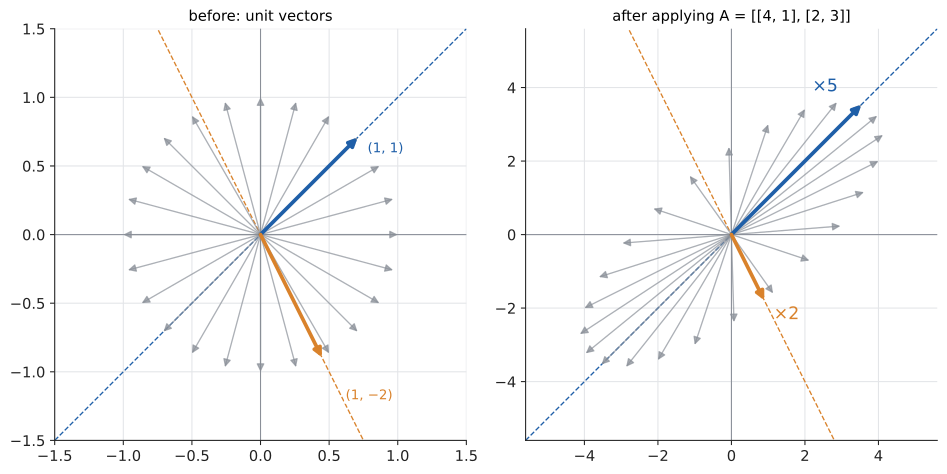
Picture the transformation acting on the whole plane. Most directions get dragged around. But a few lines through the origin are mapped onto themselves: vectors on those lines stay on them, just longer, shorter, or flipped. Those are the transformation’s natural axes, its "grain". A shear, a stretch, a projection: each has its own.

You can often spot eigenvectors from the geometry alone.

We want nonzero \(\mathbf{v}\) with \(A\mathbf{v} = \lambda\mathbf{v}\). Rewrite that with everything on one side. Since \(\lambda\mathbf{v} = \lambda I\mathbf{v}\),

Read it as a transformation: the matrix \(A - \lambda I\) sends the nonzero vector \(\mathbf{v}\) to zero. An invertible matrix can’t do that (it only sends \(\mathbf{0}\) to \(\mathbf{0}\); see Chapter 27). So \(A - \lambda I\) must be singular, which means its determinant is zero:

This is the characteristic equation. It contains only \(\lambda\), not \(\mathbf{v}\), so you can solve it for the eigenvalues first and find the eigenvectors afterwards. For a \(2\times 2\) matrix \(\begin{bmatrix} a & b \\ c & d \end{bmatrix}\),

The coefficients are two old friends: \(a + d\) is the trace (sum of the diagonal) and \(ad - bc\) is the determinant. So for any \(2\times 2\) matrix,

a quadratic, solved with the quadratic formula (Chapter 8). By the sum and product of roots, \(\lambda_1 + \lambda_2 = \operatorname{tr}A\) and \(\lambda_1\lambda_2 = \det A\), two handy checks. The second also makes geometric sense: if \(A\) stretches one direction by \(\lambda_1\) and another by \(\lambda_2\), areas scale by \(\lambda_1\lambda_2\).

Try it: Run the 2×2 procedure.

Find the eigenvalues and eigenvectors of \(A = \begin{bmatrix} 4 & 1 \\ 2 & 3 \end{bmatrix}\). Try it: Watch the eigenvectors stay put; Step through this example.

Step 1: characteristic equation. Trace \(= 4 + 3 = 7\), determinant \(= 4\cdot 3 - 1\cdot 2 = 10\).

Step 2: solve. We need two numbers with product 10 and sum 7: 5 and 2. So \((\lambda - 5)(\lambda - 2) = 0\), giving \(\lambda_1 = 5\) and \(\lambda_2 = 2\). Checks: \(5 + 2 = 7\) ✓, \(5 \times 2 = 10\) ✓.

Step 3–4: eigenvector for \(\lambda_1 = 5\).

The second row is \(-2\) times the first, as promised. The first row says \(-x + y = 0\), i.e. \(y = x\). Take \(\mathbf{v}_1 = (1, 1)\).

Eigenvector for \(\lambda_2 = 2\).

Both rows say \(2x + y = 0\), i.e. \(y = -2x\). Take \(\mathbf{v}_2 = (1, -2)\).

Step 5: check. \(A(1, 1) = (5, 5) = 5(1, 1)\) ✓ and \(A(1, -2) = (2, -4) = 2(1, -2)\) ✓. These are exactly the directions highlighted in the diagram.

Try it: Rotation: complex eigenvalues; 2I: every vector works; Shear: a defective matrix.

Try it: Run this in your browser.

We found that \(A = \begin{bmatrix} 4 & 1 \\ 2 & 3 \end{bmatrix}\) simply multiplies by 5 along \((1, 1)\) and by 2 along \((1, -2)\). That suggests a strategy: describe vectors in terms of those two directions instead of \(\mathbf{e}_1, \mathbf{e}_2\). In those coordinates, \(A\) should look like the diagonal matrix \(\begin{bmatrix} 5 & 0 \\ 0 & 2 \end{bmatrix}\). How do we switch coordinates, and what does it buy us?

Any two independent vectors form a basis of the plane (Chapter 26). Put the new basis vectors as the columns of a matrix \(P\):

If a vector has coordinates \(\mathbf{c} = (c_1, c_2)\) in the new basis, meaning it equals \(c_1(1, 1) + c_2(1, -2)\), then in standard coordinates it’s \(\mathbf{x} = P\mathbf{c}\) (that’s the column view of matrix–vector multiplication). Going the other way, \(\mathbf{c} = P^{-1}\mathbf{x}\). So:

Using the \(2\times 2\) inverse formula, \(\det P = -2 - 1 = -3\) and

Example. The vector \(\mathbf{x} = (3, 0)\) has new coordinates \(P^{-1}(3, 0) = (2, 1)\). Check: \(2(1, 1) + 1(1, -2) = (3, 0)\) ✓.

Now compute \(A\mathbf{x}\) by a detour through eigen-coordinates:

So \(A\mathbf{x} = PDP^{-1}\mathbf{x}\) for every \(\mathbf{x}\), which means

where the columns of \(P\) are eigenvectors and \(D\) is diagonal with the matching eigenvalues. Reading right to left: change to the matrix’s own coordinates, stretch along the axes, change back. A complicated-looking transformation is a diagonal one viewed in a tilted coordinate system.

Check with \(\mathbf{x} = (3, 0)\). Coordinates \((2, 1)\); scale to \((10, 2)\); back to standard: \(10(1, 1) + 2(1, -2) = (12, 6)\). Directly: \(A(3, 0) = (12, 6)\) ✓.

Here’s the payoff. Apply \(A\) twice:

The inner \(P^{-1}P\) cancels: there’s no point changing back to standard coordinates between applications. The same happens for any power:

Powers of a diagonal matrix are trivial: raise each diagonal entry to the power. So the cost of \(A^n\) no longer depends on \(n\) (beyond computing two numerical powers).

Try it: Compute A³ directly; Aⁿ by diagonalisation, live.

Check at \(n = 1\): \(\tfrac{1}{3}(12, 3; 6, 9) = (4, 1; 2, 3) = A\) ✓. At \(n = 3\): top-left \((250 + 8)/3 = 86\), top-right \((125 - 8)/3 = 39\), bottom-left \((250 - 16)/3 = 78\), bottom-right \((125 + 16)/3 = 47\). Multiplying out \(A \cdot A \cdot A\) directly gives \(\begin{bmatrix} 86 & 39 \\ 78 & 47 \end{bmatrix}\) ✓.

The formula also tells you the long-run behaviour at a glance. For large \(n\), \(5^n\) dwarfs \(2^n\), so \(A^n \approx \tfrac{5^n}{3}\begin{bmatrix} 2 & 1 \\ 2 & 1 \end{bmatrix}\): every vector gets pulled towards the \((1, 1)\) direction and grows like \(5^n\). The largest eigenvalue governs the long run. That single observation drives the next three sections.

Ecologists track animal populations by age class with a Leslie matrix. Suppose each adult produces on average 3 juveniles a year, half the juveniles survive to become adults, and half the adults survive each year. With \(\mathbf{x}_n = (j_n, a_n)\) (juveniles, adults) in year \(n\), Try it: Run the Leslie model; Leslie matrix eigenvalues.

(Trace 0.5, determinant \(0 - 1.5 = -1.5\).) For \(\lambda = 1.5\), \(L - 1.5I = \begin{bmatrix} -1.5 & 3 \\ 0.5 & -1 \end{bmatrix}\) gives \(j = 2a\), eigenvector \((2, 1)\). So in the long run the population grows by 50% a year with two juveniles for every adult, whatever it started as. The eigenvalue \(-1\) adds a boom-and-bust wobble that alternates sign each year, but relative to the \(1.5^n\) growth it shrinks by a factor \(1/1.5 = 2/3\) a year. Start with 10 adults and no juveniles: year by year the totals are 35, 32.5, 68.75, 83.1, 144.7, 197.0, and the juvenile-to-adult ratio goes \(6, 0.86, 3.2, 1.42, 2.48, 1.72, \ldots\), closing in on 2. Fisheries managers use exactly this calculation, with more age classes, to set catch limits: harvest so that the dominant eigenvalue stays at about 1.

Beyond ecology, the same "largest eigenvalue governs the long run" reasoning gives compound growth of interacting quantities in economics, the spread rate of an epidemic across age groups (the famous \(R_0\) is the dominant eigenvalue of a "next-generation matrix"), and the asymptotic running time of algorithms defined by recurrences, as the next section shows.

The Fibonacci sequence (Chapter 14) is \(F_0 = 0\), \(F_1 = 1\), \(F_{n+1} = F_n + F_{n-1}\): 0, 1, 1, 2, 3, 5, 8, 13, … Is there a formula for \(F_n\) that doesn’t require computing all the earlier terms? And how fast does the sequence grow?

The recurrence needs the two most recent terms, so track them together as a state vector \((F_{n+1}, F_n)\). One step forward:

Starting from \((F_1, F_0) = (1, 0)\), \(n\) steps give \((F_{n+1}, F_n) = M^n(1, 0)\). So the Fibonacci numbers are the entries of the powers of \(M\). (In fact \(M^n = \begin{bmatrix} F_{n+1} & F_n \\ F_n & F_{n-1} \end{bmatrix}\).)

Trace 1, determinant \(-1\), so the characteristic equation is

These are the golden ratio \(\varphi = \tfrac{1 + \sqrt{5}}{2} \approx 1.618\) and its partner \(\psi = \tfrac{1 - \sqrt{5}}{2} \approx -0.618\). Eigenvectors: for either root \(\lambda\), the vector \((\lambda, 1)\) works, because

Write the starting vector as a combination of eigenvectors. Since \(\varphi - \psi = \sqrt{5}\),

(Check: top \((\varphi - \psi)/\sqrt{5} = 1\), bottom \((1 - 1)/\sqrt{5} = 0\) ✓.) Now apply \(M^n\): each eigenvector just gets multiplied by its eigenvalue to the \(n\):

The bottom entry is

This is Binet’s formula. A sequence of whole numbers is given by a formula full of square roots of 5, which all cancel. Since \(|\psi| < 1\), the \(\psi^n\) term shrinks to nothing, so \(F_n\) is simply \(\varphi^n/\sqrt{5}\) rounded to the nearest integer, and the ratio of consecutive terms tends to \(\varphi\). The growth rate of the sequence is the dominant eigenvalue.

Binet’s formula is elegant but floating-point arithmetic ruins it for large \(n\). Matrix powers computed by repeated squaring stay in exact integers and need only about \(\log_2 n\) matrix multiplications (the same trick as fast modular exponentiation in Chapter 23): Try it: Matrix powers versus Binet’s formula.

The exact answer and the floating-point Binet answer agree in their first 14 digits and then diverge: a 64-bit float carries only about 16 significant digits (Chapter 32). Choose the method by the job: Binet for growth rates and estimates, exact matrix powers for exact values.

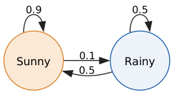
A crude weather model: if today is sunny, tomorrow is sunny with probability 0.9 and rainy with probability 0.1. If today is rainy, tomorrow is sunny or rainy with probability 0.5 each. It’s raining today. What’s the chance of sun in a week? In the long run, what fraction of days are sunny?

Let \(\mathbf{x}_n = (s_n, r_n)\) be the probabilities of sun and rain on day \(n\). Tomorrow’s chance of sun comes from two routes, sunny-then-sunny and rainy-then-sunny:

Column \(j\) of \(P\) lists where you go from state \(j\); each column sums to 1. After \(n\) days, \(\mathbf{x}_n = P^n\mathbf{x}_0\): a matrix power again.

If the distribution settles down to some \(\mathbf{x}^*\), then applying \(P\) once more leaves it unchanged: \(P\mathbf{x}^* = \mathbf{x}^*\). That’s an eigenvector with eigenvalue 1. Solve \((P - I)\mathbf{x} = \mathbf{0}\):

In the long run, five days in six are sunny, regardless of today’s weather.

Trace \(1.4\), determinant \(0.45 - 0.05 = 0.4\), so \(\lambda^2 - 1.4\lambda + 0.4 = (\lambda - 1)(\lambda - 0.4) = 0\). One eigenvalue is 1 (the steady state); the other is 0.4. Decompose the starting distribution into the steady state plus a component along the second eigenvector; each day that second component is multiplied by 0.4. So the distance from equilibrium shrinks by a factor of 0.4 per day. Starting from rain, the chance of sun on day \(n\) works out to Try it: Explore the weather chain.

which gives \(s_1 = 0.5\), \(s_2 = 0.7\), \(s_3 = 0.78\), and by day 7, \(0.8320\): within 0.002 of \(5/6\). The code confirms it:

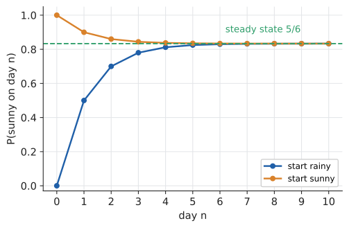
Why is 1 always an eigenvalue of a transition matrix, and why are the others no bigger than 1 in size? Because the columns sum to 1, multiplying by \(P\) preserves total probability, so no component can grow forever. The gap between 1 and the next-largest eigenvalue size (here \(1 - 0.4 = 0.6\)) is the spectral gap, and it controls the convergence speed: a big gap means the chain forgets its starting point quickly.

Try it: Watch a cycling chain.

In 1998 the web had tens of millions of pages, and keyword search returned thousands of matches for any query. Which matches should come first? Larry Page and Sergey Brin’s idea: a page is important if important pages link to it. That sounds circular, and it is. Eigenvectors are how you solve circular definitions.

Imagine a surfer who starts on a random page and, at every step, clicks a random link on the current page. Over a long time, what fraction of steps does the surfer spend on each page? Pages with many incoming links from frequently visited pages will be visited often. That long-run fraction is the page’s PageRank, and it’s exactly the steady state of a Markov chain whose states are web pages.

Here’s a tiny web:

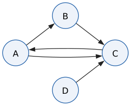
The link matrix \(M\) has \(m_{ij} = 1/(\text{number of out-links of } j)\) if page \(j\) links to page \(i\), and 0 otherwise. Columns are pages being left; each column splits its page’s "vote" equally among its links (Chapter 25 calls this a weighted adjacency matrix):

The pure random surfer gets stuck in pages with no out-links and in closed loops, and page D (no incoming links) would get rank zero, which breaks the uniqueness conditions above. The fix: with probability \(d\) (the damping factor, classically 0.85) the surfer follows a random link; with probability \(1 - d\) they get bored and jump to a page chosen uniformly at random. With \(n\) pages, the Google matrix is Try it: Move the damping slider.

where \(J\) is the matrix of all 1s. Every entry of \(G\) is positive, so the Perron–Frobenius theorem guarantees a unique steady state with all-positive entries, and the chain converges to it. The PageRank vector \(\mathbf{r}\) is the eigenvector of \(G\) with eigenvalue 1:

For the real web, \(G\) has billions of rows. You can’t run a textbook eigenvalue algorithm on it. But you don’t need to: you know the eigenvalue you want (1), you know it’s the largest, and the diagonalisation section showed that repeatedly applying a matrix swings any vector towards its dominant eigenvector. So just keep multiplying. Try it: Watch power iteration converge.

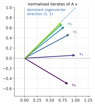
Why it works: write \(\mathbf{v}_0 = c_1\mathbf{v}_1 + c_2\mathbf{v}_2 + \cdots\) in eigenvectors. Then \(A^k\mathbf{v}_0 = c_1\lambda_1^k\mathbf{v}_1 + c_2\lambda_2^k\mathbf{v}_2 + \cdots = \lambda_1^k\big(c_1\mathbf{v}_1 + c_2(\lambda_2/\lambda_1)^k\mathbf{v}_2 + \cdots\big)\). If \(|\lambda_1|\) is strictly the largest, every ratio \((\lambda_i/\lambda_1)^k\) shrinks to zero, leaving only the \(\mathbf{v}_1\) direction. Renormalising each step stops the numbers overflowing.

Before running code, predict. D has no incoming links, so it only gets teleport traffic: \(r_D = (1 - d)/n = 0.15/4 = 0.0375\). C receives links from three pages (including all of B’s vote and all of D’s) and should rank highest. A receives all of C’s vote, so A should be close behind. B receives only half of A’s vote. Try it: Rank the tiny web; Rank the tiny web.

Check the steady-state equations by hand. Each page’s rank is its teleport share plus \(d\) times the votes it receives:

and the four ranks sum to 1. The prediction holds: C first, A a close second (one very good inbound link can be worth as much as several mediocre ones), then B, then the unlinked D.

In the exercise above, \(\begin{bmatrix} 2 & 1 \\ 1 & 2 \end{bmatrix}\) had eigenvectors \((1, 1)\) and \((1, -1)\), which are perpendicular. That’s no accident. The matrix is symmetric (\(A^\mathsf{T} = A\), Chapter 27), and symmetric matrices are the best-behaved matrices in linear algebra.

The proof is short and uses only the transpose rule \(\mathbf{u}\cdot(A\mathbf{v}) = \mathbf{u}^\mathsf{T}A\mathbf{v} = (A^\mathsf{T}\mathbf{u})^\mathsf{T}\mathbf{v}\). Suppose \(A\mathbf{u} = \lambda\mathbf{u}\) and \(A\mathbf{v} = \mu\mathbf{v}\) with \(\lambda \neq \mu\). Compute \(\mathbf{u}^\mathsf{T}A\mathbf{v}\) two ways:

The two are equal, so \((\lambda - \mu)(\mathbf{u}\cdot\mathbf{v}) = 0\). Since \(\lambda \neq \mu\), we must have \(\mathbf{u}\cdot\mathbf{v} = 0\). ∎

Symmetric matrices turn up constantly: covariance matrices (next section), the \(A^\mathsf{T}A\) of least squares, graph Laplacians, the Hessian of second derivatives (Chapter 20), and the stiffness matrices of engineering. Whenever you have one, use np.linalg.eigh, which exploits the symmetry.

You’ve measured 500 people’s height and arm span. The two numbers are strongly correlated: tall people have long arms. Plotted, the data form an elongated, tilted cloud. Is there a single number that captures most of what distinguishes one person from another? More generally, you have data with 768 features per item (embeddings, again). Can you find a handful of directions that capture most of the variation, to visualise, compress, or denoise it?

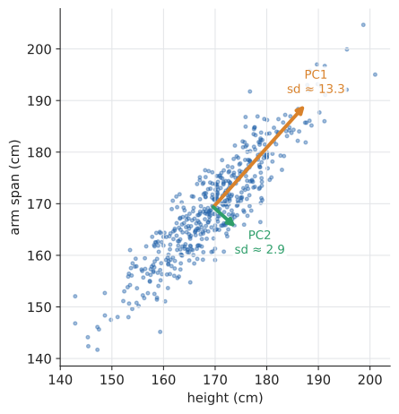
The cloud is long in one direction and thin in the other. If you projected every point onto the long axis (Chapter 26), you’d keep most of the spread between people and lose only the small sideways scatter. That long axis is the direction of maximum variance, and finding it is principal component analysis.

Centre the data (subtract the mean of each feature), so the cloud sits at the origin. Put the \(N\) centred data points as rows of a matrix \(X\) (\(N\times p\) for \(p\) features). The variance of the data projected onto a unit direction \(\mathbf{u}\) is the average of the squared projections \((\mathbf{x}_i\cdot\mathbf{u})^2\):

The matrix \(C\) is the covariance matrix (\(p\times p\), symmetric). Its diagonal entries are the variances of each feature; its off-diagonal entries are the covariances between pairs of features (Chapter 31). Now write \(C = Q\Lambda Q^\mathsf{T}\) (spectral theorem) and let \(\mathbf{y} = Q^\mathsf{T}\mathbf{u}\), the direction expressed in eigen-coordinates (still a unit vector, since \(Q^\mathsf{T}\) is a rotation):

With \(y_1^2 + \cdots + y_p^2 = 1\), this is a weighted average of the eigenvalues. It’s largest when all the weight goes on the largest eigenvalue: \(\mathbf{y} = (1, 0, \ldots, 0)\), i.e. \(\mathbf{u} = \) the top eigenvector. So:

Try it: PCA on height and arm span.

Interpret each line. The covariance matrix says height varies with variance 83.5 (standard deviation about 9.1 cm), arm span slightly more (101.3, because it adds measurement noise), and they covary strongly (83.5: arm span is height plus independent noise, so their covariance is approximately height’s own variance). The first principal component, \((0.669, 0.744)\), points roughly along the diagonal: "overall size", with both measurements increasing together. It carries 95.4% of the variance. The second, perpendicular to it, is "arms long or short for your height", with only 4.6%. So one number per person, their score on PC1, captures almost everything: two dimensions have been reduced to one with little loss. The trace checks out too: \(83.5 + 101.3 = 184.8 \approx 176.4 + 8.4\).

PCA finds linear structure. It’s the right first tool for correlated numeric features, for visualising high-dimensional data in 2D, and for compressing before another algorithm. Know its limits:

Try it: See mixed units hijack PC1.

Eigenvectors have a frustrating limitation: they only exist for square matrices (a \(3\times 2\) matrix takes 2D vectors to 3D vectors, so "\(A\mathbf{v}\) is a multiple of \(\mathbf{v}\)" makes no sense), and even square matrices may lack enough of them. Is there a decomposition that works for every matrix, of any shape?

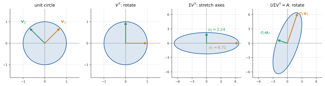
There is, and it’s the most useful factorisation in applied mathematics. Watch what a \(2\times 2\) matrix does to the unit circle: it always produces an ellipse. An ellipse has perpendicular axes. So some pair of perpendicular input directions (on the circle) must map to the perpendicular axes of the ellipse. That gives a three-step description of any matrix:

And \(A\mathbf{v}_i = \sigma_i\mathbf{u}_i\): each input axis goes to an output axis, scaled. This is the eigenvector idea generalised: you’re allowed different directions on the input and output sides, and in exchange it works for every matrix.

Find the singular values of \(A = \begin{bmatrix} 3 & 0 \\ 4 & 5 \end{bmatrix}\). Try it: SVD as rotate–stretch–rotate; Circle to ellipse, step by step.

Eigenvectors of \(A^\mathsf{T}A\) (same pattern as the \(\begin{bmatrix} 2 & 1 \\ 1 & 2 \end{bmatrix}\) exercise): \(\mathbf{v}_1 = (1, 1)/\sqrt{2}\), \(\mathbf{v}_2 = (1, -1)/\sqrt{2}\). The output directions are \(\mathbf{u}_i = A\mathbf{v}_i/\sigma_i\):

Checks: \(\mathbf{u}_1\cdot\mathbf{u}_2 = (3 - 3)/10 = 0\), both have length 1, and \(\sigma_1\sigma_2 = \sqrt{225} = 15 = |\det A|\) (area scaling is the product of the stretches). The unit circle becomes an ellipse with semi-axes 6.71 along \((1, 3)\) and 2.24 along \((3, -1)\).

Multiply out \(U\Sigma V^\mathsf{T}\) column by column and you get a sum of simple pieces:

Each term \(\mathbf{u}_i\mathbf{v}_i^\mathsf{T}\) (column times row, an outer product) is a rank-1 matrix, and the terms are ordered by importance \(\sigma_i\). Keeping only the first \(k\) terms gives a rank-\(k\) matrix \(A_k\). The Eckart–Young theorem says this truncation is the best possible rank-\(k\) approximation to \(A\): no other rank-\(k\) matrix is closer (in the sense of summed squared entry differences). And storing it takes only \(k(m + n + 1)\) numbers instead of \(mn\).

A greyscale image is just a matrix of brightness values. Here’s a synthetic 200 × 200 image (smooth waves plus a bright disc plus noise) and its low-rank approximations: Try it: Compress the image yourself.

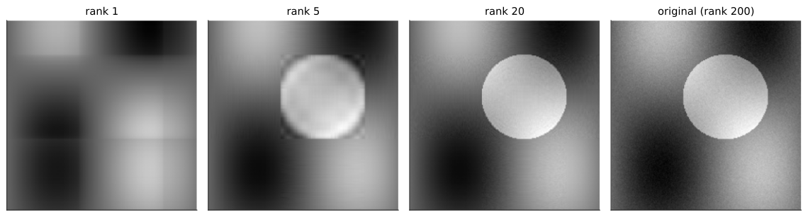
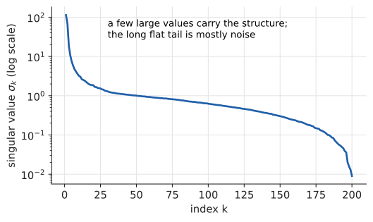
The wave part of the image, \(\sin(6x)\cos(4y)\), is a product of a function of \(x\) and a function of \(y\): exactly rank 1. That’s why the first singular value is so dominant. The disc needs a few more terms (its edges are curved, not aligned with rows and columns). Beyond about rank 20 the remaining singular values are noise, and dropping them improves the image by denoising it. Real photographs aren’t this cooperative, which is why JPEG uses a different transform (the discrete cosine transform), but the idea of "keep the big coefficients, drop the small ones" is the same.

Recall the blind spot of bag-of-words search (Chapter 26): a query for "car" scores zero against a document that only says "automobile". Latent semantic indexing (LSI, also called latent semantic analysis), introduced by Deerwester, Dumais and colleagues in 1990, fixes this with the SVD. Try it: LSI concept space.

Build the term–document matrix \(A\): one row per term, one column per document. Its rank-\(k\) approximation forces the documents into a \(k\)-dimensional "concept" space. Terms that co-occur across documents ("car", "automobile" and "engine" all appear alongside each other) end up sharing a concept direction, so documents using different words for the same thing get similar concept vectors.

Document d2 never mentions "car" and scores 0.00 on raw cosine similarity. In the 2-concept space it scores as high as the documents that do, because "automobile" and "engine" share the vehicle concept with "car". The flower documents stay at zero. (With only two clear topics, rank 2 sorts everything perfectly; real collections use \(k\) of a few hundred.)