Volume 3: Discrete and Probabilistic Mathematics · Part VI: Discrete Mathematics
Chapter 25. Graph Theory
A road map, a social network, the web, a build system, a compiler’s view of your program, and the dependency chart at the front of this book are all the same kind of object: things, and connections between them. Graph theory strips away everything else and asks what can be said about connections alone. This chapter starts with an 18th-century puzzle about bridges, builds the vocabulary (vertices, edges, degree, paths, cycles, trees), and then turns to the algorithms that make graphs useful in computing: breadth-first and depth-first search, Dijkstra’s shortest paths, topological sorting, minimum spanning trees and colouring. It ends with planar graphs and Euler’s formula, and with a glimpse of how Google ranked the web.
25.1. The bridges of Königsberg
25.1.1. The problem
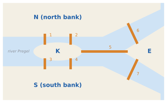
In the 1730s the Prussian city of Königsberg (now Kaliningrad, Russia) sat on both banks of the river Pregel and on an island, Kneiphof, with a fourth piece of land to the east where the river forked. Seven bridges joined the four land masses. The townspeople asked: can you take a walk that crosses every bridge exactly once? Nobody could find one, and nobody could prove it impossible.
25.1.2. Intuition: throw away the geography
In 1736 Leonhard Euler saw that almost nothing on the map matters. The size and shape of the land, the lengths of the bridges, the route you take while on dry land: all irrelevant. Only two things matter: which land masses exist and which pairs each bridge connects. So shrink each land mass to a dot and draw each bridge as a line between dots:
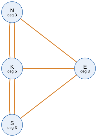
Now think about any walk that crosses each bridge once. Every time the walk passes through a land mass, it arrives on one bridge and leaves on another, using up bridges in pairs. So every land mass that is not the start or the end of the walk must touch an even number of bridges. At most two land masses (the start and the end) can have an odd number. In Königsberg, all four have an odd number (5, 3, 3, 3). So no such walk exists. No amount of trying would ever have found one. Try it: Königsberg as a graph.
That argument is the birth of graph theory, and it illustrates the subject’s power: by finding the right abstraction, a question about a city becomes a question about counting, and the answer comes with a proof. We will make it precise in Section 25.7.
|
Euler and the "geometry of position"
Euler described the problem as belonging to the geometria situs ("geometry of position") that Leibniz had imagined: a geometry where distances don’t matter, only arrangement. That idea grew into both graph theory and topology. Several of the original seven bridges were destroyed in the Second World War or demolished afterwards. Today only five bridges join these land masses, and with that layout exactly two land masses have odd degree, so an Euler path (though not a circuit) finally exists. |
25.2. Vertices, edges and the kinds of graph
25.2.1. The idea
A graph is the simplest possible model of "things and connections": a set of objects, and a set of pairs of objects that are linked.
|
Graph, vertex, edge
A graph \(G = (V, E)\) consists of a set \(V\) of vertices (also called nodes) and a set \(E\) of edges, each edge joining two vertices. An edge between \(u\) and \(v\) is written \(\{u, v\}\) or simply \(uv\). \(u\) and \(v\) are its endpoints; they are adjacent (neighbours), and the edge is incident to each of them. The number of vertices \(|V|\) is often written \(n\) and the number of edges \(|E|\) is written \(m\). The singular of vertices is vertex. "Graph" here has nothing to do with the graph of a function (Chapter 11); the word was coined by J. J. Sylvester in 1878 from "chemicograph", a diagram of molecular bonds. |
|
Kinds of graph
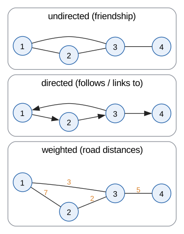
Unless stated otherwise, "graph" in this chapter means a simple undirected graph. |
25.2.2. Representing relationships as graphs
Modelling is the first skill. Ask: what are the things (vertices), and what is the relationship (edges)? Is the relationship symmetric (undirected) or not (directed)? Does it have a size (weighted)?
-
Airports and direct flights: vertices = airports, directed edges = flights, weights = fares or durations.
-
A codebase: vertices = modules, directed edge \(A \to B\) if \(A\) imports \(B\).
-
A sudoku: vertices = the 81 cells, edges between cells that may not hold the same digit.
-
A chess knight: vertices = squares, edges = legal knight moves. "Can a knight visit every square once?" is then a graph question.
A directed edge is a pair, which is exactly a relation in the sense of Chapter 21. A directed graph is a relation on \(V\), drawn as a picture; an undirected graph is a symmetric relation.
25.3. Degree and the handshake lemma
25.3.1. The problem
At a meeting, people shake hands; you ask everyone how many hands they shook and add up the answers. Can the total be odd?
25.3.2. Degree
|
Degree
The degree of a vertex \(v\), written \(\deg(v)\), is the number of edges incident to it (a loop counts twice). In a directed graph a vertex has an in-degree (arrows arriving) and an out-degree (arrows leaving). A vertex of degree 0 is isolated; a vertex of degree 1 is a leaf (or pendant vertex). A graph in which every vertex has the same degree \(k\) is \(k\)-regular. |
25.3.3. The handshake lemma
Proof (double counting). Count the pairs (vertex, edge) where the edge is incident to the vertex. Counting vertex by vertex, each vertex \(v\) contributes \(\deg(v)\) pairs, for a total of \(\sum \deg(v)\). Counting edge by edge, each edge has exactly two endpoints and contributes exactly 2 pairs, for a total of \(2|E|\). Both count the same set, so they are equal. \(\blacksquare\)
In Königsberg: \(3 + 5 + 3 + 3 = 14 = 2 \times 7\). ✓
Corollary: the number of odd-degree vertices is even. Split the sum into even-degree and odd-degree vertices. The total \(2|E|\) is even and the even-degree part is even, so the odd-degree part is even. A sum of odd numbers is even only if there is an even number of them. So the answer to the handshake question is no: the total is always even, and the number of people who shook an odd number of hands is always even.
For a directed graph the analogue is \(\sum \deg^{+}(v) = \sum \deg^{-}(v) = |E|\): every arrow leaves exactly one vertex and arrives at exactly one.
25.3.4. Worked example: is the graph possible?
Is there a simple graph with degrees \(3, 3, 3, 3, 3\)? The sum is 15, which is odd, but it must equal \(2|E|\). No.
Is there a simple graph with degrees \(4, 4, 4, 1, 1\)? The sum is 14, so it would have 7 edges, and the parity test passes. But look harder: three vertices of degree 4 in a 5-vertex simple graph must each be adjacent to every other vertex, including both degree-1 vertices. Then each degree-1 vertex would have at least 3 neighbours. Contradiction. No. The parity test is necessary, not sufficient.
25.4. Walks, paths, cycles and connectivity
25.4.1. Vocabulary
Movement through a graph has several flavours, and the words are used carefully.
|
Walk, trail, path, cycle
|
25.4.2. Connectivity
|
Connected, component
An undirected graph is connected if there is a path between every pair of vertices. Otherwise it splits into connected components: maximal connected pieces. Being "joined by a path" is an equivalence relation (reflexive, symmetric, transitive; see Chapter 21), and the components are its equivalence classes. A directed graph is strongly connected if there is a directed path from every vertex to every other, and weakly connected if it is connected when you ignore the arrows. |
A useful fact: every walk from \(u\) to \(v\) contains a path from \(u\) to \(v\). If a walk revisits a vertex, cut out the loop between the two visits; repeat until no vertex repeats. So "reachable by a walk" and "reachable by a path" mean the same thing, and the shortest walk is always a path.
|
Interactive graph sandbox
A canvas where the reader adds vertices and drags edges between them. Live panels show each vertex’s degree, the degree sum and \(2|E|\) side by side, the connected components in different colours, and whether the current graph has an Euler path, an Euler circuit, or neither, with the odd-degree vertices highlighted. Try it: Open the graph sandbox |
25.5. Trees
25.5.1. The problem
You need to connect \(n\) offices with network cable so that every office can reach every other. What is the smallest number of links that can do it, and what do minimal networks look like?
25.5.2. Intuition
Start with \(n\) isolated offices: \(n\) components. Each new link can merge at most two components into one, reducing the count by at most 1. To get down to a single component you need at least \(n - 1\) links. And a network that uses exactly \(n - 1\) has no spare links: every link is essential, so there are no cycles (a link in a cycle could be removed without disconnecting anything). Such minimal connected graphs are trees.
|
Tree, forest, leaf, rooted tree
A tree is a connected graph with no cycles. A forest is a graph with no cycles (a disjoint union of trees). A leaf is a vertex of degree 1. A rooted tree singles out one vertex as the root; then every other vertex has a unique parent (its neighbour on the path to the root) and possibly children. The depth of a vertex is its distance from the root. A spanning tree of a graph \(G\) is a tree that includes every vertex of \(G\) and uses only edges of \(G\). |
25.5.3. Why a tree on \(n\) vertices has \(n - 1\) edges
Lemma. Every tree with \(n \ge 2\) vertices has at least two leaves.
Proof. Take a longest path \(v_0, v_1, \ldots, v_k\) in the tree. Suppose \(v_0\) had a neighbour other than \(v_1\). If that neighbour were on the path, it would close a cycle; if it were off the path, it would extend the path, contradicting "longest". So \(\deg(v_0) = 1\), and by symmetry \(\deg(v_k) = 1\). \(\blacksquare\)
Theorem. A tree with \(n\) vertices has exactly \(n - 1\) edges.
Proof by induction on \(n\) (Chapter 22). For \(n = 1\), a single vertex has 0 edges. ✓ Suppose every tree with \(n - 1\) vertices has \(n - 2\) edges, and let \(T\) have \(n \ge 2\) vertices. By the lemma, \(T\) has a leaf \(\ell\). Removing \(\ell\) and its one edge leaves a graph that is still connected (no path between other vertices passed through a leaf) and still acyclic: a tree with \(n - 1\) vertices, hence \(n - 2\) edges. Putting \(\ell\) back adds one edge: \(n - 1\). \(\blacksquare\)
The following are all equivalent for a graph with \(n\) vertices; any two of the first three imply the third:
-
it is connected;
-
it has no cycles;
-
it has \(n - 1\) edges;
-
between every pair of vertices there is exactly one path.
Property 4 is why trees are the natural shape for hierarchies: file systems, the DOM, organisational charts, parse trees, and the "parent pointer" structures that BFS and DFS produce.
|
Watch the edge count
\(n - 1\) edges is not enough by itself to make a tree: a triangle plus an isolated vertex has 4 vertices and 3 edges but is neither connected nor acyclic. You need \(n - 1\) edges and one of "connected" or "acyclic". Similarly, in code, checking |
|
Counting trees
How many different trees can be built on \(n\) labelled vertices? Cayley’s formula (1889) gives the strikingly simple answer \(n^{n-2}\): 3 trees on 3 vertices, 16 on 4, 125 on 5. One elegant proof (Prüfer, 1918) encodes each tree as a sequence of \(n - 2\) vertex labels, a bijection in exactly the style of stars and bars. |
25.5.4. Where you’d use this
Chemistry: alkanes are trees. Draw a molecule with atoms as vertices and bonds as edges. An alkane \(\mathrm{C}_n\mathrm{H}_{2n+2}\) has \(3n + 2\) atoms, and its degree sum is \(4n\) (carbon) \(+ (2n + 2)\) (hydrogen) \(= 6n + 2\), so by the handshake lemma it has \(3n + 1\) bonds: exactly one fewer than its atoms. A connected graph with that many edges is a tree, so alkanes have no rings. The different isomers are the different trees the carbons can form: butane (\(n = 4\)) has 2 (a chain and a branched one), pentane has 3. Cayley’s interest in counting trees came from exactly this question.
Engineering: radial networks. Local electricity distribution networks are usually operated as trees, even when extra cables exist: with \(n\) substations and exactly \(n - 1\) closed links, there is one path from the supply to each customer, so a fault is easy to locate and isolate. Close one more link and you create a loop, which is what engineers do deliberately (and briefly) to reroute power during repairs.
Everyday and science. Family trees (going back one generation per level), company org charts, folder hierarchies and the "tree of life" in evolutionary biology are all rooted trees; a phylogenetic tree of \(n\) species, with branching ancestors as extra vertices, is built by the same "no cycles, everything connected" logic.
25.6. Bipartite graphs
25.6.1. The problem
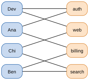
Four developers and four services: each developer can maintain certain services. Can every service get a distinct maintainer? Problems like this pair up things of two different kinds, and edges only ever run between the kinds.
|
Bipartite graph, matching
A graph is bipartite if its vertices can be split into two sets \(L\) and \(R\) (the parts) so that every edge joins a vertex of \(L\) to a vertex of \(R\). \(K_{a,b}\) is the complete bipartite graph with \(|L| = a\), \(|R| = b\) and all \(ab\) edges between them. A matching is a set of edges no two of which share an endpoint; a perfect matching covers every vertex. |
Try it: Two-colour the developer graph.
25.6.2. Recognising bipartite graphs
Theorem. A graph is bipartite if and only if it has no cycle of odd length. Try it: Watch two-colouring find odd cycles.
Why: walking round a cycle in a bipartite graph alternates sides, L, R, L, R, …, and you can only return to your starting side after an even number of steps. Conversely, if there are no odd cycles, colour a start vertex 0, its neighbours 1, their neighbours 0, and so on outward (breadth-first); a clash would mean two vertices at the same parity of distance are adjacent, which closes an odd cycle.
That proof is an algorithm. Here it is, using breadth-first search from Section 25.10:
from collections import deque

def two_colour(graph):
    """Return a 2-colouring {vertex: 0/1} if the graph is bipartite, else None."""
    side = {}
    for s in graph:                        # handle every component
        if s in side:
            continue
        side[s] = 0
        queue = deque([s])
        while queue:
            u = queue.popleft()
            for v in graph[u]:
                if v not in side:
                    side[v] = 1 - side[u]  # neighbours go on the other side
                    queue.append(v)
                elif side[v] == side[u]:   # edge inside one side: odd cycle
                    return None
    return side

square = {1: [2, 4], 2: [1, 3], 3: [2, 4], 4: [3, 1]}
triangle = {1: [2, 3], 2: [1, 3], 3: [1, 2]}
print(two_colour(square))
print(two_colour(triangle))
{1: 0, 2: 1, 4: 1, 3: 0}
None
In the developer graph above, a perfect matching exists (Ana–billing, Ben–search, Chi–web, Dev–auth, for instance). Finding maximum matchings efficiently is a classic algorithmic problem (Hopcroft–Karp, network flow) behind job assignment, ad allocation, organ-donor exchanges and medical residency placement.
25.6.3. Where you’d use this
The residency match is the famous large-scale example. Each year the US National Resident Matching Program pairs tens of thousands of newly qualified doctors with hospital training posts. The algorithm behind it finds a stable matching in a bipartite graph (no doctor and hospital would both prefer each other to what they got). Its theory, by David Gale and Lloyd Shapley, and its practice, by Alvin Roth, won the 2012 Nobel prize in economics. School-place allocation in cities such as New York and Boston uses the same algorithm. Closer to home, assigning 4 people to 4 chores they are each willing to do is a perfect-matching question, and the developer example above is the workplace version.
25.7. Euler paths and circuits
25.7.1. The problem
Return to Königsberg, generalised. Given a connected graph, can you traverse every edge exactly once? A snowplough wants to clear every street once; a pen-plotter wants to draw a figure without lifting the pen; a DNA-sequencing algorithm wants to chain overlapping fragments.
|
Euler path and Euler circuit
An Euler path (or Euler trail) is a trail that uses every edge of the graph exactly once. An Euler circuit is an Euler path that starts and ends at the same vertex. A graph with an Euler circuit is called Eulerian. |
25.7.2. The criterion
Theorem (Euler 1736, Hierholzer 1873). Let \(G\) be a connected graph (ignoring isolated vertices).
-
\(G\) has an Euler circuit if and only if every vertex has even degree.
-
\(G\) has an Euler path that is not a circuit if and only if exactly two vertices have odd degree. The path must start at one of them and end at the other.
25.7.3. Why it works
Necessity is the Königsberg argument. Each time a trail passes through a vertex, it uses one edge in and one edge out: a pair. For a circuit, the start vertex is also paired (the first edge out with the last edge in), so every degree is even. For an open path, only the two endpoints have an unpaired edge, so exactly those two have odd degree.
Sufficiency (that the condition is enough) is constructive. Start anywhere and keep walking along unused edges. With all degrees even, whenever you enter a vertex other than the start, an unused edge remains to leave by, so you can only get stuck back at the start: you have a closed trail. If it hasn’t used every edge, some vertex on it still has unused edges (the graph is connected); start a new closed trail there, using only unused edges, and splice it into the first. Repeat until every edge is used. This is Hierholzer’s algorithm, which runs in \(O(|E|)\) time. For the two-odd-vertex case, add an imaginary edge between the odd vertices, find a circuit, then delete the imaginary edge.
25.7.4. Worked example: the house
The "house" or "open envelope" puzzle asks you to draw this figure without lifting your pen or retracing a line. Try it: Trace the house’s Euler path.
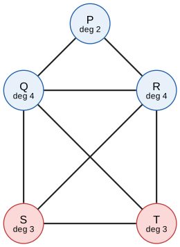
Degrees: \(P = 2\), \(Q = 4\), \(R = 4\), \(S = 3\), \(T = 3\). Sum \(16 = 2 \times 8\). ✓ Two odd vertices, so an Euler path exists and must start at S or T. One such path:
Check: 8 steps, using the edges ST, TR, RS, SQ, QR, RP, PQ, QT, which are all 8 edges, each once. Start at P instead and you will always get stuck, which is now a theorem rather than a frustration.
from collections import defaultdict

def adjacency_list(edges):
    """Build an undirected adjacency list (multi-edges allowed)."""
    adj = defaultdict(list)
    for u, v in edges:
        adj[u].append(v)
        adj[v].append(u)
    return adj

def euler_status(edges):
    adj = adjacency_list(edges)
    odd = sorted(v for v in adj if len(adj[v]) % 2 == 1)
    # (assumes the graph is connected)
    if not odd:
        return "Euler circuit exists"
    if len(odd) == 2:
        return f"Euler path exists, from {odd[0]} to {odd[1]}"
    return f"neither: {len(odd)} odd vertices {odd}"

konigsberg = [("N", "K"), ("N", "K"), ("S", "K"), ("S", "K"),
              ("N", "E"), ("K", "E"), ("S", "E")]
house = [("P", "Q"), ("P", "R"), ("Q", "R"), ("Q", "S"),
         ("Q", "T"), ("R", "S"), ("R", "T"), ("S", "T")]

adj = adjacency_list(konigsberg)
print({v: len(adj[v]) for v in adj}, sum(len(n) for n in adj.values()))
print(euler_status(konigsberg))
print(euler_status(house))
{'N': 3, 'K': 5, 'S': 3, 'E': 3} 14
neither: 4 odd vertices ['E', 'K', 'N', 'S']
Euler path exists, from S to T
|
Connectivity is part of the criterion
"All degrees even" is not enough if the graph is in two pieces: two separate triangles have all degrees 2, but no single trail covers both. Always check connectivity (for example with BFS) before applying the degree test. For a directed graph, the criterion becomes: every vertex has in-degree equal to out-degree (for a circuit), and the graph is connected when directions are ignored. |
Try it: Even degrees, two components.
25.7.5. Where you’d use this
Route planning for every street. Gritting lorries, street sweepers, postal rounds and meter readers want a closed route that covers every street, and every repeated street costs fuel. If every junction has even degree, an Euler circuit does it with no repeats. Otherwise the odd-degree junctions must be paired up and a shortest path between each pair driven twice: the Chinese postman problem, first posed by the Chinese mathematician Meigu Guan in 1960. In the house above, a sweeper that must return to its depot has to repeat one street: the S–T edge, giving 9 street-traversals for 8 streets.
Drawing machines. A pen plotter, laser cutter or CNC router drawing a connected outline wastes time on "pen-up" moves. An outline whose graph has \(2k\) odd vertices needs at least \(k\) separate strokes, so a figure with all even degrees can be cut in one continuous pass.
25.8. Hamiltonian cycles, and why they are hard
25.8.1. The problem
Change one word. Instead of using every edge once, visit every vertex once. A delivery van must call at every depot; a tour must visit every city.
|
Hamiltonian path and cycle
A Hamiltonian path visits every vertex exactly once. A Hamiltonian cycle is a Hamiltonian path that returns to its start along an edge. The weighted version, "find the cheapest Hamiltonian cycle in a complete weighted graph", is the travelling salesman problem (TSP). |
25.8.2. The contrast
The two questions look like twins, but they behave completely differently.
-
For Euler, there is a simple local test (count degrees) and a linear-time algorithm.
-
For Hamilton, no simple test is known, and none is expected. Deciding whether a graph has a Hamiltonian cycle is NP-complete: it is one of thousands of problems that are all equally hard, for which no polynomial-time algorithm is known, and for which finding one would also solve the famous P versus NP problem.
Why is the vertex version so much harder? The Euler condition is local: each vertex just needs the right parity, and the pieces can always be spliced together. Whether a vertex can be fitted into a Hamiltonian cycle depends on the global structure of the whole graph. The obvious algorithm is to try every ordering of the vertices, and there are \((n-1)!/2\) distinct cycles on \(n\) labelled vertices of a complete graph (Chapter 24). For 20 cities that is about \(6 \times 10^{16}\). Try it: Brute-force Hamiltonian cycles (cube).
There are useful sufficient conditions. Dirac’s theorem (1952): if a simple graph has \(n \ge 3\) vertices and every vertex has degree at least \(n/2\), then it has a Hamiltonian cycle. But many graphs with low degrees are Hamiltonian too (any cycle graph, for instance), so the condition is far from necessary.
25.8.3. Choosing a method in practice
For small graphs (up to about 20 vertices), exact dynamic programming over subsets (the Held–Karp algorithm, \(O(n^2 2^n)\)) is practical. For larger TSP instances, practitioners use heuristics (nearest neighbour, 2-opt improvement) and branch-and-bound solvers, which routinely solve real instances with tens of thousands of cities to optimality or near it, even though no guarantee of speed exists. "NP-hard" means "no known algorithm is fast on every input", not "hopeless in practice". Try it: Brute force vs nearest neighbour.
|
Hamilton’s puzzle
William Rowan Hamilton (who also invented quaternions, used today for 3D rotations in games) marketed the Icosian Game in 1857: find a cycle through all 20 vertices of a dodecahedron along its edges. It was a commercial flop, being rather easy, but it gave its name to one of the central hard problems of computer science. |
25.9. Representing graphs in a computer
25.9.1. The problem
To run algorithms you need a data structure. The two standard choices make different operations fast, and the right choice depends on how dense the graph is.
25.9.2. Adjacency matrix
Number the vertices \(0, \ldots, n-1\). The adjacency matrix \(A\) is the \(n \times n\) table with \(A_{ij} = 1\) if there is an edge from \(i\) to \(j\) and \(0\) otherwise (or the edge weight, for a weighted graph). For an undirected graph \(A\) is symmetric: \(A_{ij} = A_{ji}\).
For the directed graph with edges \(0 \to 1\), \(0 \to 2\), \(1 \to 2\), \(2 \to 0\), \(2 \to 3\), \(3 \to 0\):
25.9.3. Adjacency list
The adjacency list stores, for each vertex, a list of its neighbours. In Python this is naturally a dictionary of lists:
graph = {0: [1, 2], 1: [2], 2: [0, 3], 3: [0]}25.9.4. Trade-offs
| Operation | Adjacency matrix | Adjacency list |
|---|---|---|
Memory |
\(O(n^2)\) |
\(O(n + m)\) |
Is \(uv\) an edge? |
\(O(1)\): look up \(A_{uv}\) |
\(O(\deg u)\): scan the list (\(O(1)\) with a set) |
List neighbours of \(u\) |
\(O(n)\): scan a whole row |
\(O(\deg u)\) |
Visit every edge (BFS, DFS) |
\(O(n^2)\) |
\(O(n + m)\) |
Add an edge |
\(O(1)\) |
\(O(1)\) |
Linear algebra (powers, eigenvectors) |
natural |
must convert |
Choosing. Most real graphs are sparse: \(m\) is much smaller than the maximum \(\binom{n}{2}\). A social network with a billion users and a few hundred friends each has around \(10^{11}\) edges, while its adjacency matrix would have \(10^{18}\) cells, nearly all zero. Use adjacency lists by default. Use a matrix when the graph is small or dense (most pairs connected), when you need constant-time edge queries, or when you want to apply linear algebra. In numerical work, sparse matrix formats give you the memory of a list with the algebra of a matrix.
25.9.5. Powers of the adjacency matrix count walks
Here is a first taste of how matrices and graphs reinforce each other. Matrix multiplication is defined in Chapter 27; for now you need only the rule for one entry: \((A^2)_{ij} = \sum_{k} A_{ik} A_{kj}\). Try it: Count walks with powers of A.
Each term \(A_{ik}A_{kj}\) is 1 exactly when there is an edge \(i \to k\) and an edge \(k \to j\), that is, a walk \(i \to k \to j\) of length 2. The sum over all intermediate vertices \(k\) therefore counts the walks of length 2 from \(i\) to \(j\). By induction, \((A^r)_{ij}\) is the number of walks of length \(r\) from \(i\) to \(j\).
import numpy as np

# directed graph on vertices 0..3:  0->1, 0->2, 1->2, 2->0, 2->3, 3->0
A = np.array([[0, 1, 1, 0],
              [0, 0, 1, 0],
              [1, 0, 0, 1],
              [1, 0, 0, 0]])
print(A @ A)
print(np.linalg.matrix_power(A, 3))
[[1 0 1 1] [1 0 0 1] [1 1 1 0] [0 1 1 0]] [[2 1 1 1] [1 1 1 0] [1 1 2 1] [1 0 1 1]]
Check by hand. \((A^2)_{03} = 1\): the only length-2 walk from 0 to 3 is \(0 \to 2 \to 3\). \((A^3)_{00} = 2\): the two closed walks of length 3 from 0 are \(0 \to 1 \to 2 \to 0\) and \(0 \to 2 \to 3 \to 0\). The diagonal of \(A^3\) counts closed 3-walks through each vertex; in an undirected graph each triangle through a vertex gives two of them (one per direction), so the total number of triangles is \(\operatorname{trace}(A^3)/6\), a formula used in network analysis. Try it: Closed 3-walks versus triangles.
25.10. Breadth-first search
25.10.1. The problem
Given a graph and a start vertex, which vertices can you reach, and what is the fewest number of edges needed to reach each one? This is "degrees of separation", "minimum number of hops", "fewest moves to solve the puzzle".
25.10.2. Intuition: ripples in a pond
Explore in rings. First the start vertex (distance 0). Then all its neighbours (distance 1). Then all their unvisited neighbours (distance 2). And so on. A queue (first in, first out) enforces this order automatically: vertices discovered earlier are processed earlier, so you finish each ring before starting the next.
|
Queue and stack
A queue is a list where items are added at the back and removed from the front (FIFO, "first in, first out"), like people waiting in line. A stack adds and removes at the same end (LIFO, "last in, first out"), like a pile of plates. In Python, |
Input: a graph (adjacency lists) and a start vertex \(s\).
Steps:
-
Set \(\mathrm{dist}(s) = 0\), \(\mathrm{parent}(s) = \text{none}\). Put \(s\) in an empty queue. (\(s\) is now discovered.)
-
While the queue is not empty:
-
Remove the vertex \(u\) at the front of the queue.
-
For each neighbour \(v\) of \(u\) that has not been discovered: set \(\mathrm{dist}(v) = \mathrm{dist}(u) + 1\), set \(\mathrm{parent}(v) = u\), and add \(v\) to the back of the queue.
-
Output: every vertex reachable from \(s\), its distance in edges from \(s\), and a parent pointer. Following parent pointers back from any vertex gives a shortest path to it. The parent edges form a spanning tree of \(s\)'s component, the BFS tree.
25.10.3. Worked example
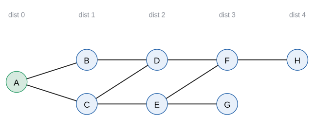
Adjacency lists (neighbours in alphabetical order): A: B, C; B: A, D; C: A, D, E; D: B, C, F; E: C, F, G; F: D, E, H; G: E; H: F. Try it: Step BFS and DFS.
| Remove | Neighbours | Newly discovered (dist, parent) | Queue afterwards |
|---|---|---|---|
A |
B, C |
B (1, A), C (1, A) |
B, C |
B |
A, D |
D (2, B) |
C, D |
C |
A, D, E |
E (2, C) (A and D already discovered) |
D, E |
D |
B, C, F |
F (3, D) |
E, F |
E |
C, F, G |
G (3, E) |
F, G |
F |
D, E, H |
H (4, F) |
G, H |
G |
E |
none |
H |
H |
F |
none |
(empty) |
Visit order: A, B, C, D, E, F, G, H. Distances: \(A{:}0\), \(B, C{:}1\), \(D, E{:}2\), \(F, G{:}3\), \(H{:}4\). A shortest path to H, read from the parent pointers backwards: \(H \leftarrow F \leftarrow D \leftarrow B \leftarrow A\), i.e. \(A, B, D, F, H\).
from collections import deque

graph = {
    "A": ["B", "C"],
    "B": ["A", "D"],
    "C": ["A", "D", "E"],
    "D": ["B", "C", "F"],
    "E": ["C", "F", "G"],
    "F": ["D", "E", "H"],
    "G": ["E"],
    "H": ["F"],
}

def bfs(graph, start):
    """Return (visit order, distance in edges, parent) from start."""
    dist = {start: 0}
    parent = {start: None}
    order = []
    queue = deque([start])
    while queue:
        u = queue.popleft()                # oldest discovered vertex
        order.append(u)
        for v in graph[u]:
            if v not in dist:              # first time we see v
                dist[v] = dist[u] + 1
                parent[v] = u
                queue.append(v)
    return order, dist, parent

def path_to(parent, target):
    path = []
    while target is not None:
        path.append(target)
        target = parent[target]
    return path[::-1]

order, dist, parent = bfs(graph, "A")
print(order)
print(dist)
print(path_to(parent, "H"))
['A', 'B', 'C', 'D', 'E', 'F', 'G', 'H']
{'A': 0, 'B': 1, 'C': 1, 'D': 2, 'E': 2, 'F': 3, 'G': 3, 'H': 4}
['A', 'B', 'D', 'F', 'H']
25.10.4. Why it works, and how fast
The queue always holds vertices of at most two consecutive distances, \(d\) then \(d + 1\), in that order. So every distance-\(d\) vertex is removed before any distance-\((d+1)\) vertex, and the first time a vertex is discovered, it is discovered from a vertex as close to \(s\) as possible. Each vertex enters the queue once and each adjacency list is scanned once, so BFS takes \(O(n + m)\) time: linear in the size of the graph.
|
Mark when discovered, not when removed
Mark a vertex as discovered when you add it to the queue, not when you take it out. Otherwise the same vertex can be added many times (once per neighbour that finds it), which wastes time and, in dense graphs, memory. And remember that BFS finds fewest edges; if edges have different weights, the path with fewest edges may not be the cheapest. That needs Dijkstra’s algorithm. |
25.11. Depth-first search
25.11.1. Intuition: explore a maze
Depth-first search is how you explore a maze with a ball of string: always go deeper down an unexplored passage; when you reach a dead end, back up to the most recent junction with an unexplored passage, and try that. Replace BFS’s queue with a stack, or use recursion (which keeps a stack for you), and you have DFS.
Input: a graph (adjacency lists) and a start vertex \(s\).
Steps:
-
Mark every vertex unvisited. Call visit(\(s\)).
-
visit(\(u\)): mark \(u\) visited and record it. For each neighbour \(v\) of \(u\), in order: if \(v\) is unvisited, call visit(\(v\)). When the loop ends, \(u\) is finished; return to the caller (backtrack).
Output: the vertices reachable from \(s\) in DFS discovery order, and (if recorded) the order in which they finish.
25.11.2. Worked trace
On the same graph, from A: Try it: DFS trace, step by step.
visit A        A's first unvisited neighbour is B
  visit B      B: A visited; go to D
    visit D    D: B visited; go to C
      visit C  C: A, D visited; go to E
        visit E      E: C visited; go to F
          visit F    F: D, E visited; go to H
            visit H  H: F visited; H finished
          F finished
          (back at E) next neighbour G
          visit G    G finished
        E finished
      C finished
    D finished
  B finished
A finished
Discovery order: A, B, D, C, E, F, H, G. Compare BFS (A, B, C, D, E, F, G, H): DFS plunged to H before ever touching G, a neighbour of E.
def dfs(graph, start):
    """Recursive depth-first search; returns vertices in discovery order."""
    visited, order = set(), []

    def visit(u):
        visited.add(u)
        order.append(u)
        for v in graph[u]:
            if v not in visited:
                visit(v)

    visit(start)
    return order

def dfs_iterative(graph, start):
    """Same idea with an explicit stack (no recursion limit)."""
    visited, order = set(), []
    stack = [start]
    while stack:
        u = stack.pop()                    # newest vertex first
        if u in visited:
            continue
        visited.add(u)
        order.append(u)
        for v in reversed(graph[u]):       # reversed: visit neighbours in listed order
            if v not in visited:
                stack.append(v)
    return order

print(dfs(graph, "A"))
print(dfs_iterative(graph, "A"))
['A', 'B', 'D', 'C', 'E', 'F', 'H', 'G'] ['A', 'B', 'D', 'C', 'E', 'F', 'H', 'G']
DFS also runs in \(O(n + m)\) time.
25.11.3. Choosing between BFS and DFS
| Need | Use | Why |
|---|---|---|
Fewest-edge paths, "degrees of separation" |
BFS |
explores in order of distance |
Just reachability, or connected components |
either |
both visit every reachable vertex once |
Detect a cycle; topological order; strongly connected components |
DFS |
finishing times expose the graph’s structure |
Explore a huge or infinite space (puzzles, game trees) with limited memory |
DFS (or iterative deepening) |
stores only the current path, not a whole frontier |
Solution likely close to the start |
BFS |
stops at the first ring that contains it |
|
Recursion depth
Python’s default recursion limit is about 1000 frames. A recursive DFS on a long path-like graph (a linked list of 100,000 nodes, say) crashes with |
|
BFS versus DFS race
Draw or load a graph (or a grid maze). Step BFS and DFS side by side from the same start, colouring vertices as discovered, in the queue/stack, and finished, with the queue or stack contents shown live. Toggle "maze mode" to see BFS flood outward in rings while DFS snakes down corridors, and compare the paths each finds to the exit. Try it: BFS versus DFS race |
25.12. Shortest paths: Dijkstra’s algorithm
25.12.1. The problem
Edges now have lengths: road distances, network latencies, costs. Find the cheapest route from a source \(S\) to every other vertex. BFS no longer works: the path with fewest edges need not be the cheapest.
25.12.2. Intuition: settle the nearest vertex first
Imagine pouring water in at \(S\), flowing along edges at constant speed. The water reaches vertices in order of their true distance. Dijkstra’s algorithm simulates this. It keeps a tentative distance for each vertex: the length of the best route found so far. At each step it takes the unfinished vertex with the smallest tentative distance and declares that distance final. Then it checks whether going through this newly finished vertex gives a shorter route to any of its neighbours, an update called relaxing an edge.
|
Relaxation
Relaxing an edge \(u \to v\) of weight \(w\) means: if \(\mathrm{dist}(u) + w < \mathrm{dist}(v)\), set \(\mathrm{dist}(v) = \mathrm{dist}(u) + w\) and \(\mathrm{parent}(v) = u\). It asks "is going via \(u\) better than the best route to \(v\) known so far?" The symbol \(\infty\) (infinity) stands for "no route found yet". |
25.12.3. Why it works
Suppose \(u\) is the unfinished vertex with smallest tentative distance \(d\). Any other route to \(u\) must leave the finished region somewhere, through some unfinished vertex \(x\) with tentative distance at least \(d\), and then continue along edges of non-negative weight. So it costs at least \(d\). Hence \(d\) is the true distance, and finalising \(u\) is safe. This is a greedy algorithm (it makes the locally best choice and never revisits it) whose correctness rests entirely on weights being non-negative.
Input: a graph with non-negative edge weights and a source \(s\).
Steps:
-
Set \(\mathrm{dist}(s) = 0\) and \(\mathrm{dist}(v) = \infty\) for every other \(v\). No vertex is finished.
-
Repeat until every reachable vertex is finished:
-
Choose the unfinished vertex \(u\) with the smallest \(\mathrm{dist}(u)\). Mark it finished.
-
For each edge \(u \to v\) with weight \(w\) where \(v\) is unfinished: relax it (if \(\mathrm{dist}(u) + w < \mathrm{dist}(v)\), update \(\mathrm{dist}(v)\) and \(\mathrm{parent}(v)\)).
-
Output: \(\mathrm{dist}(v)\), the length of a shortest path from \(s\) to each \(v\), and parent pointers from which the paths can be read backwards.
25.12.4. Fully worked trace
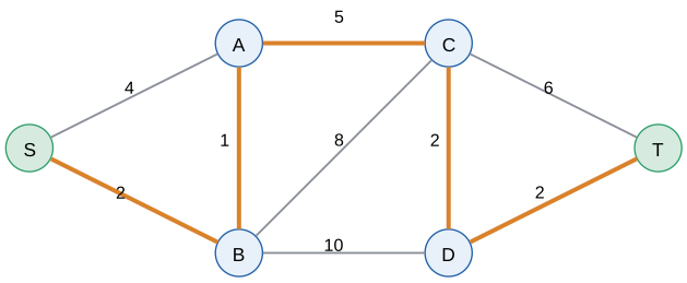
Edges (undirected): SA 4, SB 2, AB 1, AC 5, BC 8, BD 10, CD 2, CT 6, DT 2. Each cell shows the tentative distance and, in brackets, the parent. A bold entry is finalised in that step; a dash means the vertex was already finished. Try it: Step through this trace.
| Step | Finish | S | A | B | C | D | T |
|---|---|---|---|---|---|---|---|
0 |
(start) |
0 |
∞ |
∞ |
∞ |
∞ |
∞ |
1 |
S (0) |
0 |
4 (S) |
2 (S) |
∞ |
∞ |
∞ |
2 |
B (2) |
– |
3 (B) |
2 |
10 (B) |
12 (B) |
∞ |
3 |
A (3) |
– |
3 |
– |
8 (A) |
12 (B) |
∞ |
4 |
C (8) |
– |
– |
– |
8 |
10 © |
14 © |
5 |
D (10) |
– |
– |
– |
– |
10 |
12 (D) |
6 |
T (12) |
– |
– |
– |
– |
– |
12 |
Step by step:
-
Finish S (distance 0). Relax SA: \(0 + 4 = 4 < \infty\), so A becomes 4 via S. Relax SB: \(0 + 2 = 2\), B becomes 2 via S.
-
Finish B (smallest unfinished: B at 2). Relax BA: \(2 + 1 = 3 < 4\), so A improves to 3 via B. Relax BC: \(2 + 8 = 10\), C becomes 10 via B. Relax BD: \(2 + 10 = 12\), D becomes 12 via B.
-
Finish A (3). Relax AC: \(3 + 5 = 8 < 10\), C improves to 8 via A.
-
Finish C (8). Relax CD: \(8 + 2 = 10 < 12\), D improves to 10 via C. Relax CT: \(8 + 6 = 14\), T becomes 14 via C.
-
Finish D (10). Relax DT: \(10 + 2 = 12 < 14\), T improves to 12 via D.
-
Finish T (12). Done.
Read the path backwards from T using parents: \(T \leftarrow D \leftarrow C \leftarrow A \leftarrow B \leftarrow S\). The shortest route is \(S \to B \to A \to C \to D \to T\) with length \(2 + 1 + 5 + 2 + 2 = 12\). Notice that the direct-looking edge SA (4) is not on any shortest path, and that the fewest-edge route S–B–D–T (length \(2 + 10 + 2 = 14\)) loses.
import heapq

wgraph = {
    "S": {"A": 4, "B": 2},
    "A": {"S": 4, "B": 1, "C": 5},
    "B": {"S": 2, "A": 1, "C": 8, "D": 10},
    "C": {"A": 5, "B": 8, "D": 2, "T": 6},
    "D": {"B": 10, "C": 2, "T": 2},
    "T": {"C": 6, "D": 2},
}

def dijkstra(graph, source):
    """Shortest-path distances and parents from source (weights >= 0)."""
    dist = {source: 0}
    parent = {source: None}
    done = set()
    heap = [(0, source)]                      # (tentative distance, vertex)
    while heap:
        d, u = heapq.heappop(heap)            # closest unfinished vertex
        if u in done:
            continue                          # stale entry; skip it
        done.add(u)
        for v, w in graph[u].items():
            if v in done:
                continue                      # finished vertices are never revisited
            new = d + w
            if v not in dist or new < dist[v]:   # relax edge u -> v
                dist[v] = new
                parent[v] = u
                heapq.heappush(heap, (new, v))
    return dist, parent

dist, parent = dijkstra(wgraph, "S")
print(dist)
path, v = [], "T"
while v is not None:
    path.append(v)
    v = parent[v]
print(path[::-1])
{'S': 0, 'A': 3, 'B': 2, 'C': 8, 'D': 10, 'T': 12}
['S', 'B', 'A', 'C', 'D', 'T']
The priority queue (heapq, a binary heap) finds the smallest tentative distance in \(O(\log n)\) time instead of scanning every vertex. Rather than updating entries inside the heap, the code pushes a new entry on every improvement and skips "stale" entries when they surface. The total running time is \(O((n + m)\log n)\).
25.12.5. Failure mode: negative weights
Take vertices S, A, B with edges \(S \to A\) (weight 2), \(S \to B\) (weight 3) and \(B \to A\) (weight \(-2\)). Dijkstra finishes A first at distance 2, because it is the nearest unfinished vertex, and never reconsiders it. But \(S \to B \to A\) costs \(3 - 2 = 1\). The greedy argument broke because a later edge could reduce a total. Try it: Watch the negative edge fool Dijkstra.
25.12.6. Alternative approaches and choosing a method
| Situation | Algorithm | Time |
|---|---|---|
Unweighted (all edges cost 1) |
BFS |
\(O(n + m)\) |
Non-negative weights, one source |
Dijkstra |
\(O((n + m) \log n)\) |
One source and one target, with a good distance estimate (maps, games) |
A* search (Dijkstra guided by a heuristic) |
often far less than Dijkstra |
Negative weights allowed; detect negative cycles |
Bellman–Ford |
\(O(nm)\) |
Shortest paths between all pairs, small dense graph |
Floyd–Warshall |
\(O(n^3)\) |
Directed acyclic graph |
relax edges in topological order |
\(O(n + m)\) |
|
Dijkstra and the shortest-path problem
Edsger Dijkstra designed the algorithm in 1956 in about twenty minutes, sitting at a café terrace in Amsterdam with his fiancée, without pencil or paper. He wanted a demonstration problem for a new computer, the ARMAC, that non-mathematicians could understand: the shortest route between two Dutch cities. He later remarked that designing without pencil and paper was one reason the algorithm turned out so simple: it forces you to avoid all avoidable complexities. |
|
Dijkstra step-through
Load the example graph or draw your own. Step through Dijkstra’s algorithm, with finished vertices shaded, tentative distances shown on each vertex, and each relaxation flashing the edge involved. The trace table above fills in row by row. A "negative edge" toggle lets the reader set one weight below zero and watch the algorithm confidently report a wrong answer. Try it: Dijkstra step-through |
25.12.7. Where you’d use this
Navigation. A phone’s route planner runs a refined Dijkstra (A* search plus precomputed shortcuts called contraction hierarchies) on road graphs with tens of millions of junctions. The weights are travel times, not distances, which is why "fastest" and "shortest" routes differ. Public-transport journey planners do the same on a graph whose vertices are (stop, time) pairs.
Finance: spotting arbitrage. Exchange rates multiply along a path, but shortest-path algorithms add. Taking logarithms fixes that: give the edge from currency \(X\) to \(Y\) the weight \(-\ln(\text{rate})\). Suppose USD \(\to\) EUR is 0.90, EUR \(\to\) GBP is 0.90 and GBP \(\to\) USD is 1.25. Round the cycle, $1 becomes \(0.90 \times 0.90 \times 1.25 = 1.0125\) dollars, and the weights sum to \(-\ln 1.0125 < 0\): a negative cycle. Bellman–Ford (the table above) detects negative cycles, which is why it, not Dijkstra, is the textbook tool for this. (Real markets close such gaps within milliseconds.) Try it: Find the arbitrage cycle.
Networks. Internet routers inside one organisation run OSPF, which is Dijkstra on the link-state graph, recomputed whenever a link fails.
25.13. Dependency graphs and topological sort
25.13.1. The problem
Some tasks must happen before others. A course has prerequisites; a source file must be compiled before the program that links it; a package must be installed before the packages that depend on it. Given all the "must come before" constraints, find an order that respects every one of them.
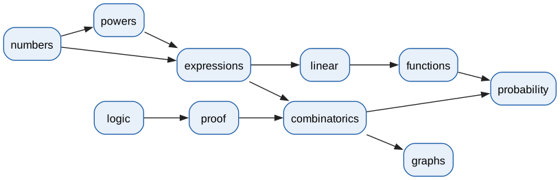
This book is itself an example. The map at the front (The Knowledge Map) is a directed graph whose edges say "read this chapter first". Here is a fragment:
|
DAG and topological order
A directed acyclic graph (DAG) is a directed graph with no directed cycle. A topological order (or topological sort) of a directed graph is a listing of all its vertices such that for every edge \(u \to v\), \(u\) comes before \(v\). A vertex with in-degree 0 is a source; with out-degree 0, a sink. |
Theorem. A directed graph has a topological order if and only if it is a DAG.
If there is a cycle \(v_1 \to v_2 \to \cdots \to v_k \to v_1\), then \(v_1\) must come before itself, which is impossible. Conversely, every DAG has a source (follow edges backwards from any vertex; with no cycles and finitely many vertices you must reach a vertex with no incoming edge). Put a source first, delete it, and the rest is still a DAG; repeat. That argument is Kahn’s algorithm.
Input: a directed graph.
Steps:
-
Compute the in-degree of every vertex (how many unmet prerequisites it has).
-
Put every vertex of in-degree 0 into a set ready.
-
While ready is not empty: remove a vertex \(u\) from it and append \(u\) to the output. For each edge \(u \to v\), decrease \(v\)'s in-degree by 1; if it reaches 0, add \(v\) to ready.
-
If the output contains every vertex, it is a topological order. If not, the remaining vertices all lie on or behind a cycle: report it.
Output: a topological order, or a proof that none exists.
25.13.2. Worked trace
In-degrees at the start: numbers 0, logic 0, powers 1, expressions 2, linear 1, functions 1, proof 1, combinatorics 2, graphs 1, probability 2. When several vertices are ready, take them alphabetically (any choice gives a valid order). Try it: Step through Kahn’s algorithm.
| Take | In-degree changes | Ready afterwards |
|---|---|---|
(start) |
logic, numbers |
|
logic |
proof 1→0 |
numbers, proof |
numbers |
powers 1→0, expressions 2→1 |
powers, proof |
powers |
expressions 1→0 |
expressions, proof |
expressions |
linear 1→0, combinatorics 2→1 |
linear, proof |
linear |
functions 1→0 |
functions, proof |
functions |
probability 2→1 |
proof |
proof |
combinatorics 1→0 |
combinatorics |
combinatorics |
graphs 1→0, probability 1→0 |
graphs, probability |
graphs |
probability |
|
probability |
(empty) |
Order: logic, numbers, powers, expressions, linear, functions, proof, combinatorics, graphs, probability. Every arrow points forward.
import heapq

# edge u -> v means "u must come before v"
prereqs = {
    "numbers":       ["powers", "expressions"],
    "powers":        ["expressions"],
    "expressions":   ["linear", "combinatorics"],
    "linear":        ["functions"],
    "functions":     ["probability"],
    "logic":         ["proof"],
    "proof":         ["combinatorics"],
    "combinatorics": ["graphs", "probability"],
    "graphs":        [],
    "probability":   [],
}

def topological_sort(graph):
    """Kahn's algorithm. Ties broken alphabetically for a reproducible order."""
    indegree = {u: 0 for u in graph}
    for u in graph:
        for v in graph[u]:
            indegree[v] += 1
    ready = [u for u in graph if indegree[u] == 0]   # no unmet prerequisites
    heapq.heapify(ready)
    order = []
    while ready:
        u = heapq.heappop(ready)
        order.append(u)
        for v in graph[u]:                 # u is done: v has one fewer blocker
            indegree[v] -= 1
            if indegree[v] == 0:
                heapq.heappush(ready, v)
    if len(order) < len(graph):
        raise ValueError("graph has a cycle; no topological order exists")
    return order

print(topological_sort(prereqs))
prereqs["graphs"].append("logic")          # introduce a cycle
try:
    topological_sort(prereqs)
except ValueError as e:
    print(e)
Try it: Add the cycle, watch it stall.
['logic', 'numbers', 'powers', 'expressions', 'linear', 'functions', 'proof', 'combinatorics', 'graphs', 'probability']
graph has a cycle; no topological order exists
Alternative method. Run DFS and list vertices in order of finishing time, then reverse the list. A vertex finishes only after everything reachable from it has finished, so in the reversed list it comes before all of its descendants. Both methods are \(O(n + m)\). Kahn’s algorithm is easier to explain, naturally reports cycles, and shows which tasks can run in parallel (everything in ready at the same moment); the DFS method is shorter to code when you already have DFS.
|
Topological orders are rarely unique
A DAG usually has many valid topological orders (here, "numbers" could equally have gone before "logic"). Code that silently depends on one particular order, for instance a build that happens to work only because two independent steps ran in a fixed sequence, will break when the tie-breaking changes. If two tasks really must be ordered, add the edge. |
25.13.3. Where you’d use this
Project planning: the critical path. A small building job has five tasks: foundation (3 weeks), then walls (4 weeks) and plumbing (2 weeks), roof after the walls (2 weeks), and finishing after both roof and plumbing (1 week). Any topological order is a valid schedule. The shortest possible project length is the longest path through the DAG: foundation \(\to\) walls \(\to\) roof \(\to\) finishing, \(3 + 4 + 2 + 1 = 10\) weeks. Plumbing lies on a path of only \(3 + 2 + 1 = 6\) weeks, so it has 4 weeks of slack; a delay on the critical path delays the whole job. Engineers call this the critical path method, and it was developed in the late 1950s to schedule large construction and defence projects. Try it: Find the critical path.
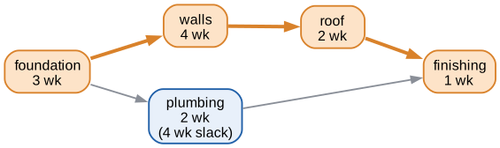
Everyday. A recipe is a DAG: you cannot sauté onions you have not chopped, but you can boil the water while you chop. Reading the steps as a dependency graph tells you what can happen in parallel and which step sets the time the meal is ready.
25.14. Minimum spanning trees
25.14.1. The problem
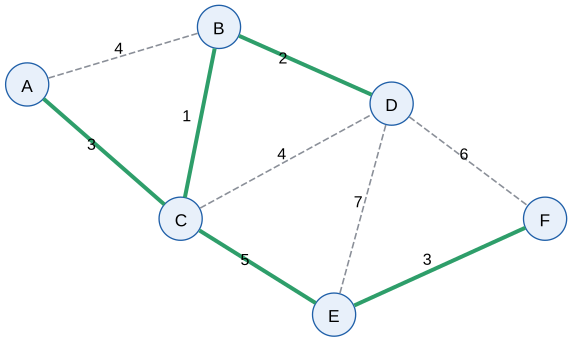
You must connect six sites with fibre. Each possible link has a cost. Every site must be able to reach every other (possibly indirectly), and you want the cheapest network. By Section 25.5, a cheapest such network has no cycles (removing a cycle edge saves money and keeps everything connected), so it is a spanning tree: a minimum spanning tree (MST).
25.14.2. Kruskal’s algorithm
Sort the edges from cheapest to dearest. Take each edge in turn, and keep it unless it would form a cycle with the edges already kept. Stop when you have \(n - 1\) edges.
Input: a connected weighted graph with \(n\) vertices.
Steps:
-
Sort all edges by weight, smallest first.
-
Start with each vertex in its own component and an empty tree.
-
For each edge \(uv\) in sorted order: if \(u\) and \(v\) are in different components, add \(uv\) to the tree and merge their components; otherwise skip it (it would close a cycle).
-
Stop when the tree has \(n - 1\) edges.
Output: a minimum spanning tree.
Worked trace (edges: BC 1, BD 2, AC 3, EF 3, AB 4, CD 4, CE 5, DF 6, DE 7): Try it: Step through Kruskal.
| Edge | Decision | Components afterwards |
|---|---|---|
BC 1 |
keep |
{B, C}, {A}, {D}, {E}, {F} |
BD 2 |
keep |
{B, C, D}, {A}, {E}, {F} |
AC 3 |
keep |
{A, B, C, D}, {E}, {F} |
EF 3 |
keep |
{A, B, C, D}, {E, F} |
AB 4 |
skip: A, B already connected |
unchanged |
CD 4 |
skip: C, D already connected |
unchanged |
CE 5 |
keep (5th edge = \(n - 1\); stop) |
{A, B, C, D, E, F} |
Total weight \(1 + 2 + 3 + 3 + 5 = 14\).
edges = [  # (weight, u, v)
    (4, "A", "B"), (3, "A", "C"), (1, "B", "C"), (2, "B", "D"),
    (4, "C", "D"), (5, "C", "E"), (7, "D", "E"), (6, "D", "F"), (3, "E", "F"),
]

def kruskal(vertices, edges):
    parent = {v: v for v in vertices}      # union-find forest

    def find(v):                           # root of v's component
        while parent[v] != v:
            parent[v] = parent[parent[v]]  # path halving
            v = parent[v]
        return v

    tree = []
    for w, u, v in sorted(edges):          # cheapest edges first
        ru, rv = find(u), find(v)
        if ru != rv:                       # joins two components: no cycle
            parent[ru] = rv
            tree.append((u, v, w))
    return tree

mst = kruskal("ABCDEF", edges)
print(mst, sum(w for _, _, w in mst))
[('B', 'C', 1), ('B', 'D', 2), ('A', 'C', 3), ('E', 'F', 3), ('C', 'E', 5)] 14
The "same component?" test uses a union–find (disjoint-set) structure, which answers it in nearly constant time; sorting dominates, so Kruskal runs in \(O(m \log m)\).
Why greedy works here (the cut property). Split the vertices into any two groups. The cheapest edge crossing between the groups belongs to some MST: if a spanning tree avoided it, adding it would create a cycle that crosses the split at least twice, and swapping out the other, dearer crossing edge would give a tree that is no more expensive. Every edge Kruskal keeps is the cheapest edge crossing between its own component and the rest, so every choice is safe.
25.14.3. Prim’s algorithm, briefly
Prim’s algorithm grows a single tree from a start vertex: repeatedly add the cheapest edge joining the tree to a vertex not yet in it. It is Dijkstra’s algorithm with one change (the priority of a vertex is the weight of the single edge connecting it, not the total path length) and runs in \(O((n + m)\log n)\) with a heap. Choosing: Kruskal is simple and natural when edges arrive as a list; Prim suits dense graphs and adjacency structures. Both give a minimum total weight; if several edges have equal weights, different MSTs of the same total can result. Try it: Grow the tree with Prim.
|
An MST is not a shortest-path tree
A minimum spanning tree minimises the total cost of the network, not the distance between any particular pair. In the MST above, A to E costs \(3 + 5 = 8\) along the tree, but if the graph had a direct A–E edge of weight 7 it would not be in the MST, and the shortest A–E route would use it. Pick MST when you’re paying to build every link once (cabling, pipelines, clustering); pick shortest paths when you’re paying per trip (routing). |
25.14.4. Where you’d use this
Infrastructure. The first MST algorithm was published in 1926 by Otakar Borůvka for a practical problem: designing an economical electricity network for southern Moravia. Treat the example graph above as possible cable routes between six villages with lengths in kilometres. Laying every route would cost \(4 + 3 + 1 + 2 + 4 + 5 + 7 + 6 + 3 = 35\) km of cable; the MST connects all six villages with 14 km. Pipelines, fibre networks and irrigation channels are planned the same way, usually as a starting point before adding a few redundant links for resilience.
Science and data. Biologists and data scientists build an MST on the pairwise distances between samples and then delete its longest edges; the pieces that remain are clusters (single-linkage clustering). The same trick groups similar images, documents or customer records.
Algorithms. For the travelling salesman problem (Section 25.8) with ordinary distances, walking around an MST and skipping repeated cities gives a tour at most twice the optimal length, a quick guaranteed-quality answer to an intractable problem.
25.15. Graph colouring
25.15.1. The problem
Six exams must be scheduled. Two exams that share a student cannot be in the same time slot. What is the smallest number of slots?
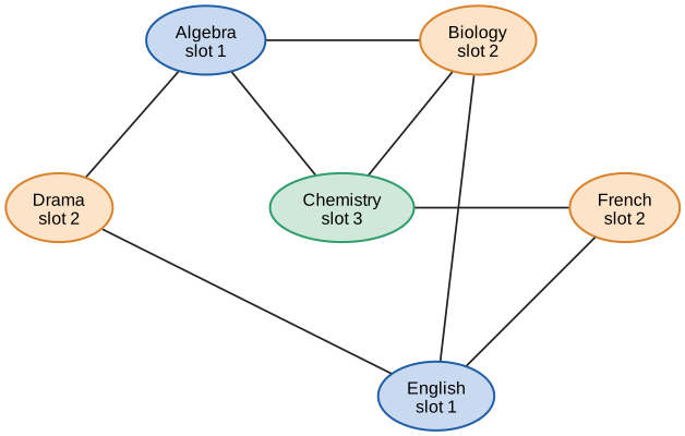
Build a conflict graph: one vertex per exam, an edge when two exams share a student. A schedule is an assignment of slots to vertices with adjacent vertices in different slots. Call the slots colours, and this is graph colouring.
|
Graph colouring and chromatic number
A (proper) colouring of a graph assigns a colour to each vertex so that adjacent vertices get different colours. The chromatic number \(\chi(G)\) (Greek letter chi) is the fewest colours that suffice. \(\chi(G) \le 2\) exactly when \(G\) is bipartite; \(\chi(K_n) = n\); a graph containing a triangle needs at least 3. |
25.15.2. The greedy method
Go through the vertices in some order and give each the smallest colour not already used by a coloured neighbour. Try it: Greedy-colour the exams.
Input: a graph and an ordering of its vertices.
Steps:
-
For each vertex \(u\) in the given order: collect the colours already used by \(u\)'s coloured neighbours, and give \(u\) the smallest colour number (0, 1, 2, …) not in that collection.
Output: a proper colouring using at most \(\Delta + 1\) colours, where \(\Delta\) is the largest degree (each vertex has at most \(\Delta\) neighbours blocking colours).
def greedy_colouring(graph, order):
    """Give each vertex, in the given order, the smallest colour not used by
    an already-coloured neighbour. Colours are 0, 1, 2, ..."""
    colour = {}
    for u in order:
        taken = {colour[v] for v in graph[u] if v in colour}
        c = 0
        while c in taken:
            c += 1
        colour[u] = c
    return colour

# exams that share a student cannot be in the same slot
conflicts = {
    "Algebra":   ["Biology", "Chemistry", "Drama"],
    "Biology":   ["Algebra", "Chemistry", "English"],
    "Chemistry": ["Algebra", "Biology", "French"],
    "Drama":     ["Algebra", "English"],
    "English":   ["Biology", "Drama", "French"],
    "French":    ["Chemistry", "English"],
}
c = greedy_colouring(conflicts, list(conflicts))
print(c, max(c.values()) + 1)

# a bipartite "crown" graph where a bad order wastes colours
crown = {f"a{i}": [f"b{j}" for j in range(1, 5) if j != i] for i in range(1, 5)}
crown.update({f"b{j}": [f"a{i}" for i in range(1, 5) if i != j] for j in range(1, 5)})
bad = ["a1", "b1", "a2", "b2", "a3", "b3", "a4", "b4"]
good = ["a1", "a2", "a3", "a4", "b1", "b2", "b3", "b4"]
print(max(greedy_colouring(crown, bad).values()) + 1,
      max(greedy_colouring(crown, good).values()) + 1)
{'Algebra': 0, 'Biology': 1, 'Chemistry': 2, 'Drama': 1, 'English': 0, 'French': 1} 3
4 2
Trace for the exams: Algebra gets 0. Biology is adjacent to Algebra (0), so gets 1. Chemistry is adjacent to Algebra (0) and Biology (1), so gets 2. Drama is adjacent to Algebra (0): gets 1. English is adjacent to Biology (1) and Drama (1): gets 0. French is adjacent to Chemistry (2) and English (0): gets 1. Three slots, and the Algebra–Biology–Chemistry triangle proves three is optimal.
25.15.3. Failure mode: greedy depends on the order
The second test colours a crown graph (each \(a_i\) joined to every \(b_j\) with \(j \ne i\)). It is bipartite, so 2 colours suffice, and greedy finds 2 when it colours all the \(a\)'s first. But in the interleaved order \(a_1, b_1, a_2, b_2, \ldots\), greedy uses 4; with \(k\) pairs it would use \(k\). Finding \(\chi(G)\) exactly is NP-hard (even deciding whether 3 colours suffice), so practical systems use good heuristic orders (largest degree first, or DSatur, which colours the most-constrained vertex next) and accept near-optimal answers. Try it: Greedy in a bad order.
25.15.4. Applications
-
Scheduling: exams, meetings, sports fixtures, with conflicts as edges and time slots as colours.
-
Register allocation: a compiler builds an interference graph whose vertices are program variables and whose edges join variables that are live at the same time. Colours are CPU registers. If the graph can’t be coloured with the available registers, some variables are "spilled" to memory. Chaitin’s 1981 register allocator made this the standard approach.
-
Frequency assignment: radio transmitters that are close together (edges) need different frequencies (colours).
-
Sudoku is a 9-colouring of an 81-vertex graph with some colours pre-assigned.
-
Map colouring: countries are vertices, shared borders are edges.
|
The four-colour theorem
In 1852 Francis Guthrie noticed that he could colour a map of the counties of England with four colours so that neighbouring counties differed, and asked whether four always suffice. The question resisted proof for 124 years. In 1976 Kenneth Appel and Wolfgang Haken proved that every planar map can be four-coloured, by reducing the problem to 1,936 configurations checked by computer. It was the first major theorem proved with essential computer assistance, and it provoked a long debate about whether a proof that no human can check by hand counts as a proof. A formally verified version (Gonthier, 2005, in the Coq proof assistant) has since settled most doubts. |
25.16. Planar graphs and Euler’s formula
25.16.1. The problem
Three houses must each be connected to three utilities (water, gas, electricity) by pipes that do not cross. Can it be done on flat ground? Circuit designers ask the same question: can this circuit be laid out on a single layer without wires crossing?
|
Planar graph, face
A graph is planar if it can be drawn in the plane with no edges crossing. Such a drawing is a plane embedding. The edges divide the plane into regions called faces, including one unbounded outer face. A planar graph can also have non-planar drawings; planarity asks whether some crossing-free drawing exists. |
25.16.2. Euler’s formula
For any connected plane graph with \(V\) vertices, \(E\) edges and \(F\) faces,
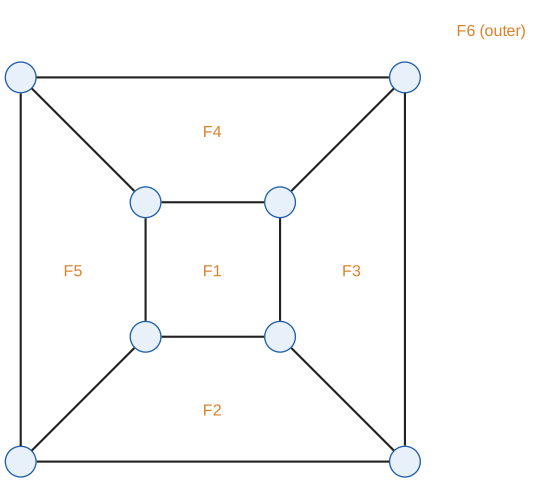
Proof by induction on the number of edges. If the graph is a tree, it has no cycles, so there is only the outer face: \(F = 1\), and \(E = V - 1\) (Section 25.5), giving \(V - (V - 1) + 1 = 2\). ✓ If it is not a tree, it has a cycle. Remove one edge of that cycle. The graph stays connected (the rest of the cycle still joins the two endpoints), and the two faces on either side of that edge merge into one. So \(E\) and \(F\) each drop by 1, and \(V - E + F\) is unchanged. Repeat until a tree remains, where the value is 2. \(\blacksquare\)
The cube itself (as a solid) has 8 corners, 12 edges and 6 faces, and \(8 - 12 + 6 = 2\): this is Euler’s polyhedron formula, of which the graph version is a flattened form. Every convex polyhedron obeys it.
25.16.3. Consequence: an edge limit, and the utilities puzzle
In a simple planar graph with \(V \ge 3\), every face is bounded by at least 3 edges, and every edge borders at most 2 faces. Counting (edge, face) border pairs both ways gives \(3F \le 2E\). Substitute \(F = 2 - V + E\) from Euler’s formula:
\(K_5\) is not planar. It has \(V = 5\) and \(E = \binom{5}{2} = 10\), but \(3V - 6 = 9 < 10\). Try it: Test K5 for planarity.
\(K_{3,3}\) (three houses, three utilities) is not planar. It is bipartite, so it has no triangles, and every face has at least 4 edges. The same counting gives \(4F \le 2E\), hence \(E \le 2V - 4 = 2 \times 6 - 4 = 8\). But \(K_{3,3}\) has \(3 \times 3 = 9\) edges. The puzzle is impossible. Try it: Test K3,3 for planarity.
These two graphs are, in a precise sense, the only obstacles. Kuratowski’s theorem (1930): a graph is planar if and only if it does not contain a subdivision of \(K_5\) or \(K_{3,3}\). Linear-time planarity-testing algorithms exist (Hopcroft and Tarjan, 1974).
|
The edge test only proves non-planarity
\(E \le 3V - 6\) is a necessary condition. A graph that satisfies it may still be non-planar (\(K_{3,3}\) satisfies \(9 \le 12\), which is why you need the sharper triangle-free bound). Use the inequality to rule planarity out quickly; never to rule it in. Also, Euler’s formula as stated needs the graph to be connected; with \(c\) components it becomes \(V - E + F = 1 + c\). |
25.17. A teaser: PageRank
How should a search engine decide which of a million matching web pages is most important? Larry Page and Sergey Brin’s 1998 answer was to use the link graph: a page is important if important pages link to it. That sounds circular, and it is, in the way that eigenvector equations are. Try it: Run this PageRank example.
Imagine a random surfer who, at each step, follows a random outgoing link from the current page with probability \(d = 0.85\), or jumps to a page chosen uniformly at random with probability \(0.15\). Over a long time, the fraction of time spent on each page settles down to a fixed distribution: that is the PageRank. If \(M\) is the matrix whose column \(i\) spreads page \(i\)'s score equally over the pages it links to, the scores \(\mathbf{r}\) satisfy
and you can find \(\mathbf{r}\) by simply iterating that equation:
import numpy as np

# links[i] = pages that page i links to
links = {0: [1, 2], 1: [2], 2: [0], 3: [2]}
n, d = 4, 0.85                         # d: probability of following a link

M = np.zeros((n, n))
for i, outs in links.items():
    for j in outs:
        M[j, i] = 1 / len(outs)        # column i spreads page i's score

r = np.full(n, 1 / n)                  # start with equal scores
for _ in range(100):
    r = (1 - d) / n + d * M @ r        # follow a link, or jump at random
print(np.round(r, 3))
[0.373 0.196 0.394 0.038]
Page 2, linked from three pages, ranks highest. Page 0 ranks second even though only one page links to it, because that one page (page 2) is itself important and gives page 0 all of its score. Page 3, which nothing links to, gets only the random-jump share. Why the iteration converges, and why the answer is an eigenvector of a matrix built from the graph, is the story of Chapter 28; the random surfer is a Markov chain, met again in Chapter 29.
25.18. Interactive tools
Browser tools on the companion website that go with this chapter. Each example link in the chapter opens one of them with that example already set up.
25.19. Exercises
-
(Recognition) A simple graph has 10 vertices, each of degree 3. How many edges does it have? Could a simple graph have 9 vertices, each of degree 3?
-
(Recognition) Which of these are trees? (a) 6 vertices, 5 edges, connected. (b) 6 vertices, 5 edges, containing a cycle. (c) 6 vertices, 6 edges, connected.
-
(Application) For the graph with edges AB, AC, BC, BD, CD, DE, decide whether it has an Euler circuit, an Euler path, or neither. If a path exists, give one. Try it: Check your Euler answer.
-
(Application) Run BFS from vertex 1 on the graph with adjacency lists 1: [2, 3], 2: [1, 4, 5], 3: [1, 5], 4: [2, 6], 5: [2, 3, 6], 6: [4, 5]. Give the visit order and the distance of each vertex. Try it: Check your BFS answer.
-
(Application) Run Dijkstra’s algorithm from A on the directed graph with edges A→B 7, A→C 2, C→B 3, B→D 1, C→D 8, D→E 2, C→E 10. Show the table of tentative distances and give the shortest path to E. Try it: Check your Dijkstra answer.
-
(Application) Find a topological order of the tasks:
fetchbeforecompile;configurebeforecompile;compilebeforetestandpackage;testbeforedeploy;packagebeforedeploy. How many tasks can run in parallel at the first step? Try it: Check your build order. -
(Problem solving) A connected planar simple graph has 10 vertices, each of degree 3. How many faces does any plane drawing of it have?
-
(Problem solving) Prove that in any graph with at least 2 vertices, two vertices have the same degree. (Hint: Chapter 24.)
-
(Problem solving, CS) You store a road network with 50 million intersections and 120 million road segments. Estimate the memory of an adjacency matrix (1 bit per entry) versus adjacency lists (8 bytes per stored neighbour entry, each segment stored twice). Which do you choose?
Answers
-
Handshake lemma: \(2|E| = 10 \times 3 = 30\), so \(|E| = 15\). With 9 vertices the degree sum would be \(27\), which is odd and cannot equal \(2|E|\): impossible.
-
(a) Yes: connected with \(n - 1\) edges. (b) No: a tree has no cycles (such a graph must also be disconnected). (c) No: a tree on 6 vertices has exactly 5 edges.
-
Degrees: A 2, B 3, C 3, D 3, E 1. Four odd vertices (B, C, D, E): neither.
-
Queue process: remove 1 → discover 2, 3; remove 2 → discover 4, 5; remove 3 → (5 already found); remove 4 → discover 6; remove 5, remove 6. Order 1, 2, 3, 4, 5, 6. Distances: 1:0, 2:1, 3:1, 4:2, 5:2, 6:3.
-
Init A0, others ∞. Finish A (0): B 7 (A), C 2 (A). Finish C (2): B min(7, 2+3=5) = 5 ©; D 2+8 = 10 ©; E 2+10 = 12 ©. Finish B (5): D min(10, 5+1=6) = 6 (B). Finish D (6): E min(12, 6+2=8) = 8 (D). Finish E (8). Path: \(A \to C \to B \to D \to E\), length \(2 + 3 + 1 + 2 = 8\).
-
In-degree 0 at the start:
configure,fetch, so 2 tasks can run in parallel. One order: configure, fetch, compile, package, test, deploy (package and test can also run in parallel once compile finishes). -
\(E = 10 \times 3 / 2 = 15\). Euler: \(F = 2 - V + E = 2 - 10 + 15 = 7\).
-
A simple graph on \(n\) vertices has degrees in \(\{0, 1, \ldots, n-1\}\): \(n\) values. But 0 and \(n-1\) cannot both occur (a vertex adjacent to all others rules out an isolated vertex). So at most \(n - 1\) distinct values are available for \(n\) vertices; by the pigeonhole principle two share a degree. (This is the handshake puzzle from Chapter 24.)
-
Matrix: \((5 \times 10^7)^2 = 2.5 \times 10^{15}\) bits \(\approx 3.1 \times 10^{14}\) bytes, about 312 TB. Lists: \(2 \times 1.2 \times 10^8 \times 8 \approx 1.9 \times 10^9\) bytes, about 2 GB, plus a small per-vertex overhead. Adjacency lists, by a factor of over 100,000: the graph is extremely sparse (average degree under 5).
25.20. Mastery check
-
State the handshake lemma and use it to show that a 7-vertex graph cannot have every vertex of degree 5.
-
A graph has degrees 2, 2, 4, 4, 3, 3 and is connected. Does it have an Euler circuit, an Euler path or neither? Between which vertices?
-
Why can BFS find shortest paths in an unweighted graph but not in a weighted one? Which algorithm do you use instead, and what condition on the weights does it need?
-
Run Dijkstra from S on: S–A 1, S–B 5, A–B 2, A–C 6, B–C 1. Give final distances.
-
Your package manager reports "circular dependency". Which algorithm detected it, and what property of the dependency graph failed?
-
Find the weight of a minimum spanning tree of the complete graph on vertices P, Q, R, S with weights PQ 1, PR 3, PS 4, QR 2, QS 5, RS 6.
-
Show that \(K_5\) is not planar.
-
A compiler has 6 variables whose live ranges pairwise overlap for every pair except (a, f). How many registers are needed to avoid spilling?
Decision rule: All correct without hesitation → move on to Chapter 26, with matrices and Chapter 28 (PageRank) to come. Stuck on 1–2 → reread the relevant section (Section 25.12 and Section 25.7 cause the most trouble). Stuck on more → work the chapter exercises, and trace BFS and Dijkstra by hand on a small graph of your own before running the code.
Mastery check answers
-
\(\sum \deg(v) = 2|E|\). With 7 vertices of degree 5 the sum is 35, which is odd: impossible.
-
Exactly two odd vertices (the two of degree 3), and the graph is connected, so an Euler path exists, starting at one degree-3 vertex and ending at the other. No Euler circuit.
-
BFS processes vertices in order of number of edges from the start, which equals distance only when every edge costs the same. With weights, a path of more, cheaper edges can be shorter. Use Dijkstra’s algorithm, which requires non-negative weights (otherwise Bellman–Ford).
-
Finish S (0): A 1, B 5. Finish A (1): B min(5, 3) = 3, C 7. Finish B (3): C min(7, 4) = 4. Finish C (4). Distances: S 0, A 1, B 3, C 4.
-
A topological sort (e.g. Kahn’s algorithm) failed to place every package: the dependency graph is not acyclic. It contains a directed cycle, so no install order satisfies every dependency.
-
Kruskal: PQ 1 (keep), QR 2 (keep), PR 3 (skip, cycle), PS 4 (keep). Three edges for 4 vertices: weight \(1 + 2 + 4 = 7\).
-
\(V = 5\), \(E = \binom{5}{2} = 10\). A simple planar graph with \(V \ge 3\) has \(E \le 3V - 6 = 9\). Since \(10 > 9\), \(K_5\) is not planar.
-
The interference graph is \(K_6\) minus the edge af. Vertices b, c, d, e and a form \(K_5\), so at least 5 colours are needed; a and f are not adjacent, so they can share a colour, and 5 suffice. Five registers.